Lab 6 - Poisson - Answers

Author

Jason Geller

To complete this lab:

Load packages

library(MASS)
library(tidyverse)
library(emmeans)
library(ggeffects)
library(easystats)
library(performance)
library(knitr)

Download the dataset:

library(tidyverse)

data <- read_delim("https://raw.githubusercontent.com/jgeller112/psy504-advanced-stats/main/slides/Poisson/data/2010.csv")

Conduct the analysis described in the preregistration document

The number of hours per week that a person spends on the Internet (“WWWHR”) will
be predicted by their vocabulary (“WORDSUM”), age (“AGE”), sex (“SEX”), religiosity
(“RELITEN”), political orientation (“POLVIEWS”), and how often they work from home
(“WRKHOME”).

data_pos <- data %>%
  dplyr::select(wwwhr, wordsum, age, sex, reliten, polviews, wrkhome) %>%
  mutate(wwwhr=case_when(
    wwwhr==-1 ~ NA_real_, 
    wwwhr==998 ~ NA_real_, 
    wwwhr==999 ~ NA_real_,
    TRUE ~ wwwhr), 
    wordsum=case_when(
    wordsum==-1 ~ NA_real_,
    wordsum==99 ~ NA_real_, 
    TRUE ~ wordsum), 
    case_when(
    reliten==0 ~ NA_real_, 
    reliten==8 ~ NA_real_, 
    reliten==9 ~ NA_real_, 
    TRUE~reliten), 
    polviews=case_when(
    polviews==0 ~ NA_real_, 
    polviews==8 ~ NA_real_, 
    polviews==9 ~ NA_real_, 
    TRUE ~ polviews), 
    wrkhome=case_when(
    wrkhome==0 ~ NA_real_, 
    wrkhome==8 ~ NA_real_, 
    wrkhome==9 ~ NA_real_, 
    TRUE ~ wrkhome), 
    age = case_when(
    age == 0 ~ NA_real_,
    age == 98 ~ NA_real_,
    age == 99 ~ NA_real_,
    TRUE ~ age))

NANIAR

could use the naniar function replace_with_na

library(naniar)

data_pos <- data %>%
  dplyr::select(wwwhr, wordsum, age, sex, reliten, polviews, wrkhome) %>%
replace_with_na(.,
             replace = list(wwwhr = c(-1, 998, 999),
                          wordsum = c(-1, 99),
                          reliten = c(0, 8, 9), 
             polviews = c(0, 8, 9), 
             wrkhome = c(0,8,9), 
             age=c(0, 98, 99)))

Recode sex as factor

data_pos <- data_pos %>%
  mutate(sex=as.factor(sex))

Recode reliten

::: {.cell}

data_pos <- data_pos %>%
  mutate(reliten_recode = case_when(
    reliten==3 ~2, 
    reliten==2 ~ 3, 
    TRUE ~ reliten
  ))

data_pos %>%
  dplyr::select(reliten, reliten_recode)

::: {.cell-output .cell-output-stdout}

# A tibble: 2,044 × 2
   reliten reliten_recode
     <dbl>          <dbl>
 1       1              1
 2       4              4
 3       1              1
 4       1              1
 5       1              1
 6       4              4
 7       3              2
 8       1              1
 9       1              1
10       1              1
# ℹ 2,034 more rows

::: :::

Missingness

library(skimr)
skimr::skim(data_pos)

Data summary
Name	data_pos
Number of rows	2044
Number of columns	8
_______________________
Column type frequency:
factor	1
numeric	7
________________________
Group variables	None

Variable type: factor

skim_variable	n_missing	complete_rate	ordered	n_unique	top_counts
sex	0	1	FALSE	2	-1: 1153, 1: 891

Variable type: numeric

skim_variable	n_missing	complete_rate	mean	sd	p0	p25	p50	p75	p100	hist
wwwhr	996	0.51	9.79	13.41	0	2	5	14	168	▇▁▁▁▁
wordsum	657	0.68	6.03	2.07	0	5	6	7	10	▁▃▇▅▂
age	3	1.00	47.97	17.68	18	33	47	61	89	▇▇▇▅▃
reliten	99	0.95	2.08	1.08	1	1	2	3	4	▇▇▁▂▃
polviews	71	0.97	4.08	1.46	1	3	4	5	7	▃▂▇▃▅
wrkhome	882	0.57	2.26	1.72	1	1	1	4	6	▇▁▁▂▁
reliten_recode	99	0.95	2.39	1.16	1	1	3	3	4	▇▂▁▇▃

Fit Poisson

pos_mod <- glm(wwwhr~wordsum+age+sex+reliten_recode+polviews+wrkhome, family=poisson(), data=data_pos)

Checking Assumptions

Performance - `check_model`

check_model(pos_mod)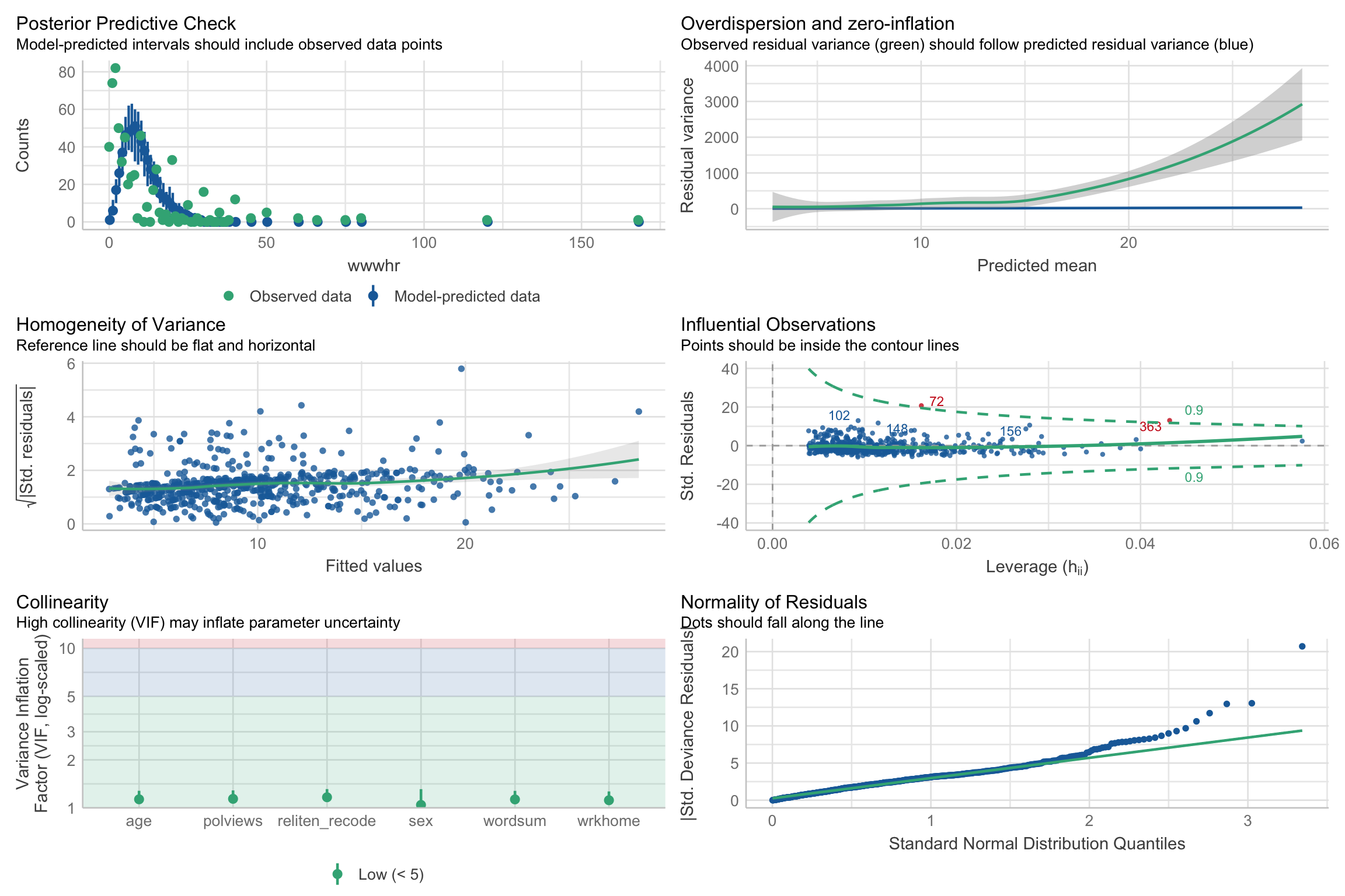

outliers_list <- check_outliers(pos_mod) # Find outliers
outliers_list # Show the row index of the outliers

2 outliers detected: cases 72, 363.
- Based on the following method and threshold: cook (0.9).
- For variable: (Whole model).

outliers_list <- as.numeric(outliers_list) # The object is a binary vector...

filtered_data <- as.data.frame(data_pos)[!outliers_list, ] # And can be used to filter a dataframe

Refit after outlier exclusion

pos_mod <- glm(wwwhr~wordsum+age+sex+reliten_recode+polviews+wrkhome, family=poisson, data=filtered_data)

model_parameters(pos_mod) %>%
  print_html()

Parameter	Coefficient	SE	95% CI	z	p
(Intercept)	1.56	0.09	(1.39, 1.72)	18.19	< .001
wordsum	0.11	7.72e-03	(0.09, 0.12)	13.76	< .001
age	-0.02	1.08e-03	(-0.02, -0.02)	-16.11	< .001
sex (1)	0.25	0.03	(0.20, 0.30)	9.35	< .001
reliten recode	0.21	0.01	(0.18, 0.23)	16.02	< .001
polviews	-0.04	9.75e-03	(-0.06, -0.02)	-3.77	< .001
wrkhome	0.08	7.67e-03	(0.07, 0.10)	10.50	< .001

Overdispersion

library(performance)

check_overdispersion(pos_mod)

# Overdispersion test

       dispersion ratio =   14.732
  Pearson's Chi-Squared = 8750.592
                p-value =  < 0.001

Our model appears to be over-dispersed. Let’s fit a negative binomial!
Let’s check if the negative binomial solved are problem:

library(MASS)

pos_mod_nb <- glm.nb(wwwhr~wordsum+age+sex+reliten_recode+polviews+wrkhome, data=filtered_data)

model_parameters(pos_mod_nb) %>%
  print_html()

Parameter	Coefficient	SE	95% CI	z	p
(Intercept)	1.66	0.28	(1.12, 2.21)	6.00	< .001
wordsum	0.11	0.03	(0.05, 0.16)	4.19	< .001
age	-0.02	3.50e-03	(-0.02, -0.01)	-4.91	< .001
sex (1)	0.16	0.09	(-0.02, 0.34)	1.79	0.073
reliten recode	0.20	0.04	(0.12, 0.27)	4.81	< .001
polviews	-0.04	0.03	(-0.10, 0.03)	-1.10	0.270
wrkhome	0.06	0.03	(7.36e-03, 0.12)	2.25	0.025

Which one is better?

test_likelihoodratio(pos_mod, pos_mod_nb)

# Likelihood-Ratio-Test (LRT) for Model Comparison (ML-estimator)

Name       |  Model | df | df_diff |    Chi2 |      p
-----------------------------------------------------
pos_mod    |    glm |  7 |         |         |       
pos_mod_nb | negbin |  8 |       1 | 4606.62 | < .001

Negative binom appears to be better!

check_zeroinflation(pos_mod_nb)

# Check for zero-inflation

   Observed zeros: 40
  Predicted zeros: 67
            Ratio: 1.68

No zero-inflation!

Log Lambda
Mean Count

model_parameters(pos_mod_nb) %>%
  print_html()

Parameter	Coefficient	SE	95% CI	z	p
(Intercept)	1.66	0.28	(1.12, 2.21)	6.00	< .001
wordsum	0.11	0.03	(0.05, 0.16)	4.19	< .001
age	-0.02	3.50e-03	(-0.02, -0.01)	-4.91	< .001
sex (1)	0.16	0.09	(-0.02, 0.34)	1.79	0.073
reliten recode	0.20	0.04	(0.12, 0.27)	4.81	< .001
polviews	-0.04	0.03	(-0.10, 0.03)	-1.10	0.270
wrkhome	0.06	0.03	(7.36e-03, 0.12)	2.25	0.025

model_parameters(pos_mod_nb, exponentiate = TRUE) %>%
  print_html()

Parameter	Coefficient	SE	95% CI	z	p
(Intercept)	5.26	1.46	(3.06, 9.09)	6.00	< .001
wordsum	1.11	0.03	(1.06, 1.18)	4.19	< .001
age	0.98	3.44e-03	(0.98, 0.99)	-4.91	< .001
sex (1)	1.17	0.11	(0.98, 1.41)	1.79	0.073
reliten recode	1.22	0.05	(1.12, 1.32)	4.81	< .001
polviews	0.96	0.03	(0.90, 1.03)	-1.10	0.270
wrkhome	1.06	0.03	(1.01, 1.12)	2.25	0.025

The analysis employed a negative binomial regression model in R to examine the relationship between sex, age, vocabulary, religious and political views, and time spent on the internet per hour. An over-dispersion test was conducted using the performance package in R to determine the appropriateness of the model.

The analysis revealed that each additional point in the vocabulary test was associated with an increase of 11% in the expected count of hours spent on the internet per week, incidence rate ratio (IRR) = 1.11, SE = .01, p < .001. Increases in religiosity and work-from-home frequency were also associated with increased time spent on the internet, IRR = 1.10, SE = .03, p < .001, and IRR = 1.06, SE = .02, p < .001, respectively. Relative to females, males in our dataset spent more hours online, IRR = 1.28, SE = .05, p < .001, d = 1.28. Two variables, age and political orientation, were negatively associated with time spent on the internet. Older respondents and the more politically conservative spent less time online, IRR = .98, SE = .002, p < .001, d = .98, and IRR = .96, SE = .02, p = .01, d = .96, respectively.