Multilevel Modeing (with R) Part 2

Princeton University

Jason Geller, PH.D.(he/him)

2024-02-07

Multilevel models

When to use them:
- Nested designs
- Repeated measures
- Longitudinal data
- Complex designs
Why use them:
- Captures variance occurring between groups and within groups
What they are:
- Linear model with extra residuals

Today

Everything you need to know to run and report a MLM
- Organizing data for MLM analysis
- Estimation
- Fit and interpret multilevel models
- Visualization
- Effect size
- Reporting
- Power

Packages

library(tidyverse) # data wrangling
library(knitr) # nice tables
library(lme4) # fit mixed models
library(lmerTest) # mixed models
library(broom.mixed) # tidy output of mixed models
library(afex) # fit mixed models for lrt test
library(emmeans) # marginal means
library(ggeffects) # marginal means
library(ggrain) # rain plots
library(easystats) # nice ecosystem of packages

options(scipen=999) # get rid of sci notation

Find the .qmd document here to follow along: https://github.com/jgeller112/PSY504-Advanced-Stats-S24/blob/main/slides/02-MLM/mlm-02.qmd

Today’s data

What did you say?
- Ps (N = 31) listened to both clear (NS) and 6 channel vocoded speech (V6)
  - (https://www.mrc-cbu.cam.ac.uk/personal/matt.davis/vocode/a1_6.wav)
    - Fixed factor: ?
    - Random factor: ?

Today’s data

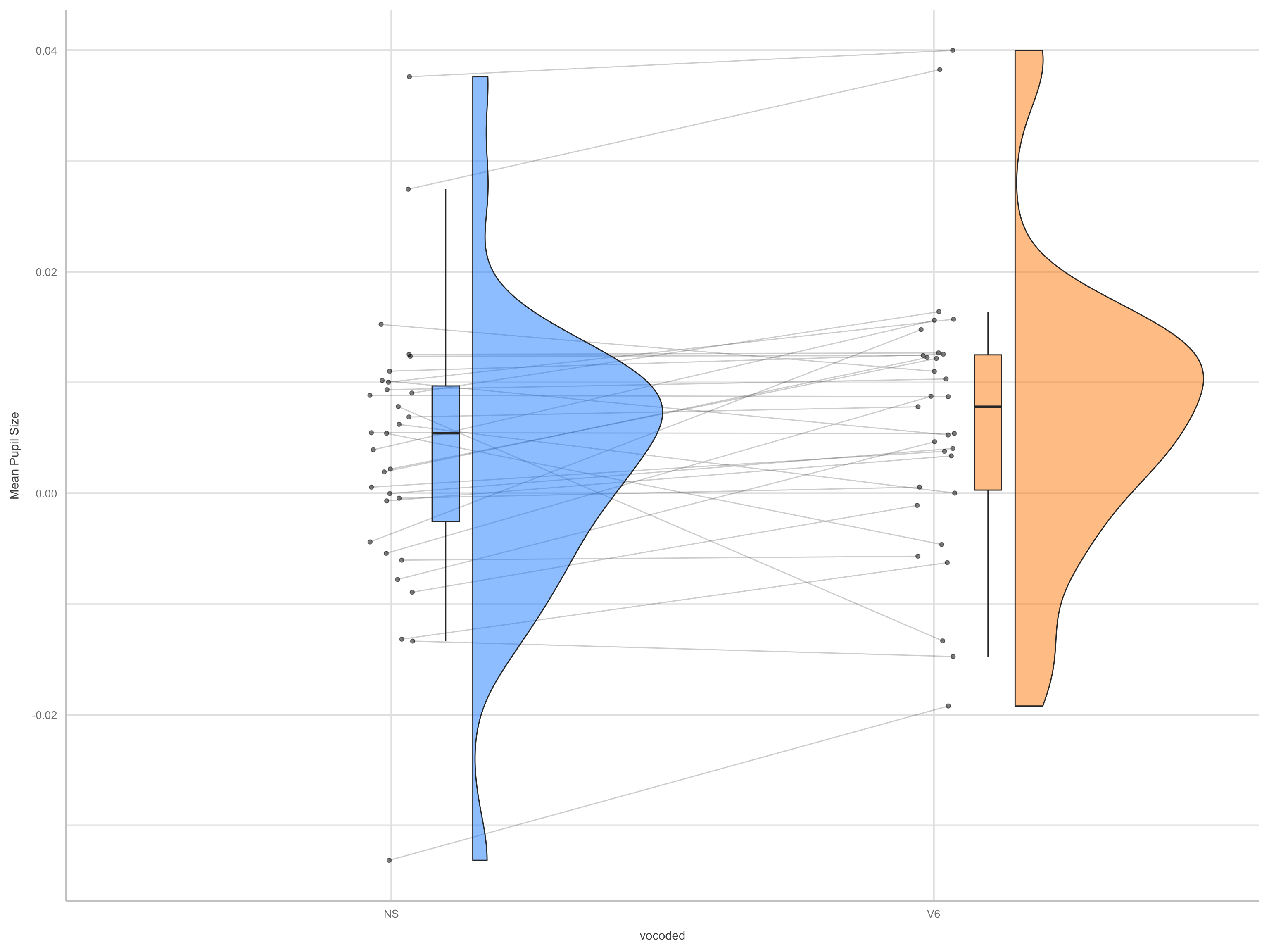
eye  <- read_csv("https://raw.githubusercontent.com/jgeller112/psy504-advanced-stats/main/slides/MLM/data/vocoded_pupil.csv") # data for class

Data organization

Data Structure
- MLM analysis (in R) requires data in long format

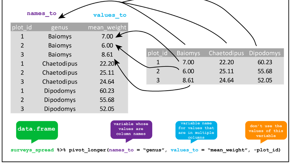
Data organization

Level 1: trial
Level 2: subject

subject	trial	vocoded	mean_pupil
EYE15	3	V6	0.0839555
EYE15	4	V6	0.0141083
EYE15	5	V6	0.0224967
EYE15	6	V6	0.0007424
EYE15	7	V6	0.0242540
EYE15	8	V6	0.0267617

Centering

In a single-level regression, centering ensures that the zero value for each predictor is meaningful before running the model
In MLM, if you have specific questions about within, between, and contextual effects, you need to center!

Group- vs. Grand-Mean Centering

Grand-mean centering: \(x_{ij} - x\)
- Variable represents each observation’s deviation from everyone’s norm, regardless of group
Group-mean centering: \(x_{ij} - x_j\)
- Variable represents each observation’s deviation from their group’s norm (removes group effect)

Group- vs. Grand-Mean Centering

Level 1 predictors
- Grand-mean centering
  - Include means of level 2
    - Allows us to directly test within-group effect
    - Coefficient associated with the Level 2 group mean represents contextual effect

Group-mean centering
- Level 1 coefficient will always be with within-group effect, regardless of whether the group means are included at Level 2 or not
- If level 2 means included, coefficient represents the between-groups effect

Note

Can apply to categorical predictors as well (see Yaremych, Preacher, & Hedeker, 2023)

Centering in R

# how to group mean center 
d <- d %>% 
  # Grand mean centering (CMC)
  mutate(iv.gmc = iv-mean(iv)) %>%
  # group  mean centering (more generally, centering within cluster)
  group_by(id) %>% 
  mutate(iv.cm = mean(iv),
         iv.cwc = iv-iv.cm)

library(datawizard) #easystats 

#data wizard way
x <- demean(x, select=c("x"), group="ID") #gets within-group and included cluster means

Model Estimation

Maximum Likelihood

In MLM we try to maximize the likelihood of the data
- No OLS!

Probability vs. Likelihood

Probability

If I assume a distribution with certain parameters (fixed), what is the probability I see a particular value in the data?

Pr⁡(𝑦>0│𝜇=0,𝜎=1)=.50
Pr⁡(−1<𝑦<1│𝜇=0,𝜎=1)=.68
Pr⁡(0<𝑦<1│𝜇=0,𝜎=1)=.34
Pr⁡(𝑦>2│𝜇=0,𝜎=1)=.02

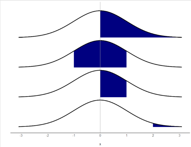
Likelihood

\(L(𝜇,𝜎│𝑥)\)
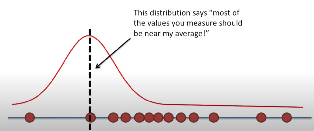
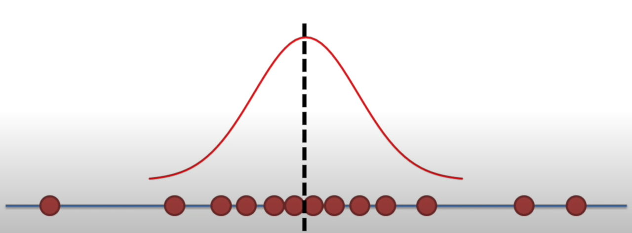
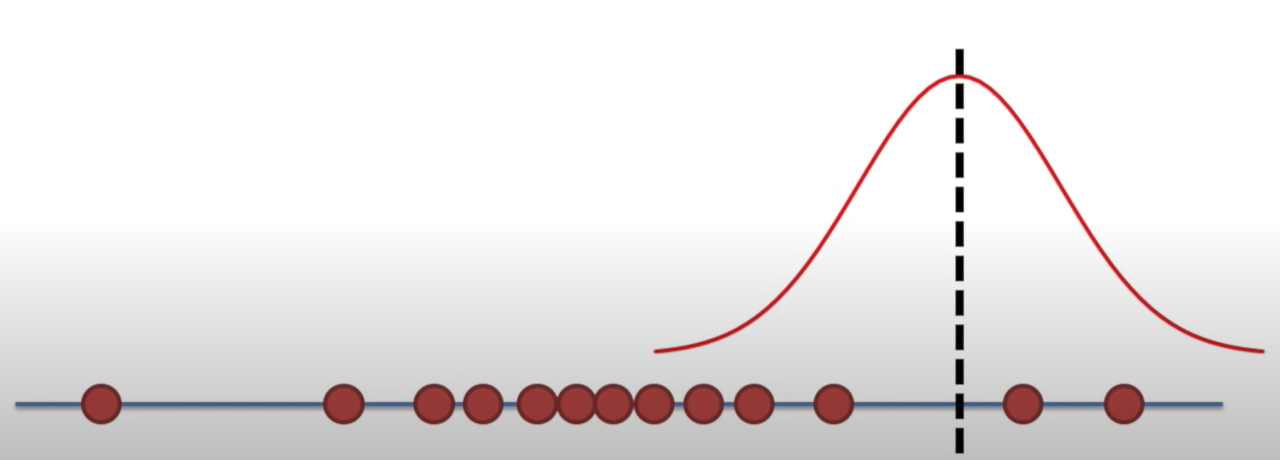
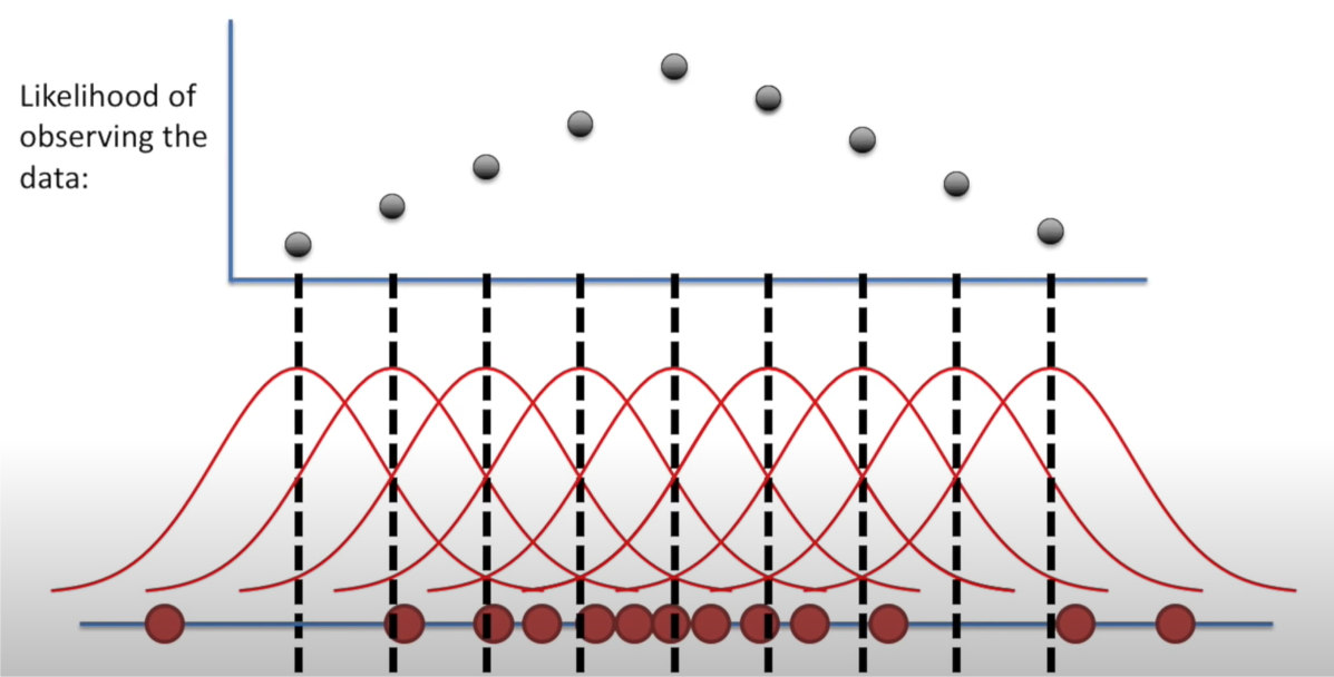
Holding a sample of data constant, which parameter values are more likely?
- Which values have higher likelihood?
Here data is fixed and distribution can change

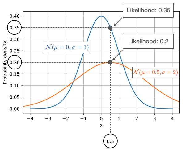
Likelihood

Interactive: Understanding Maximum Likelihood Estimation: https://rpsychologist.com/likelihood/

Log likelihood

With large samples, likelihood values ℒ(𝜇,𝜎│𝑥) get very small very fast
- To make them easier to work with, we usually work with the log-likelihood
  - Measure of how well the model fits the data
  - Higher values of \(\log L\) are better
Deviance = \(-2logL\)
- \(-2logL\) follows a \(\chi^2\) distribution with \(n (\text{sample size}) - p (\text{paramters}) - 1\) degrees of freedom

\(\chi^2\) distribution

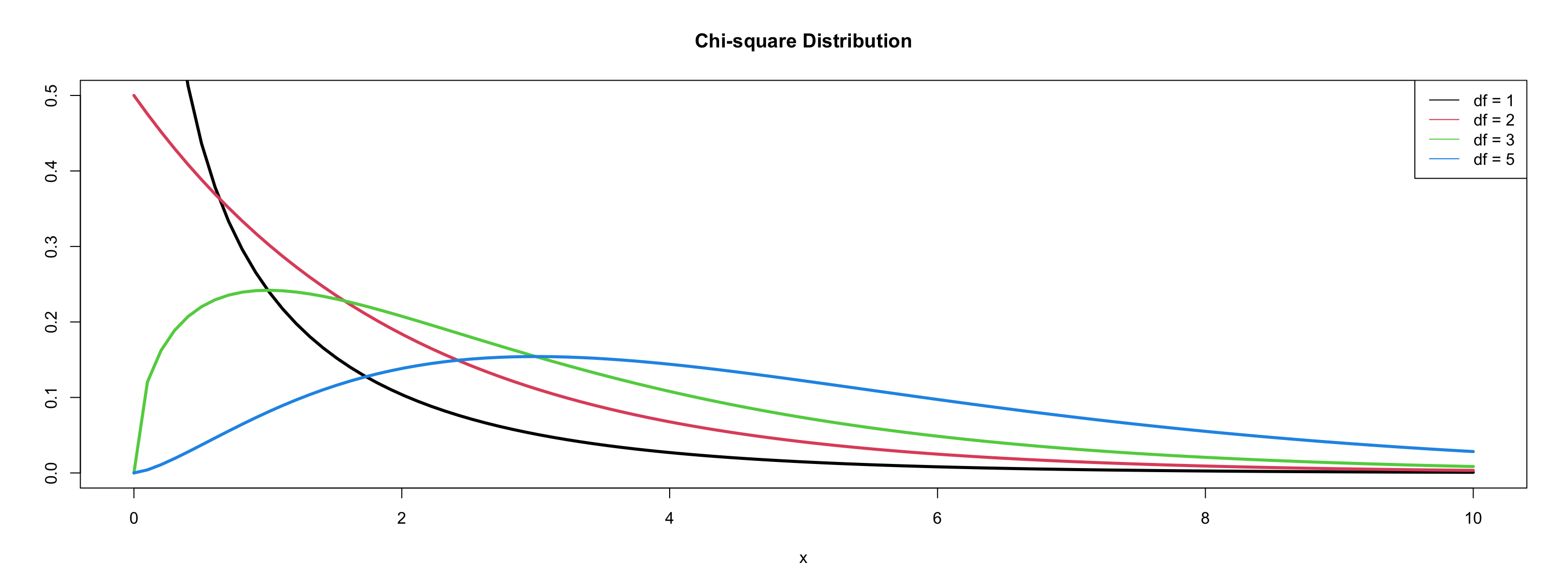
Comparing nested models

Suppose there are two models:
- Reduced model includes predictors \(x_1, \ldots, x_q\)
- Full model includes predictors \(x_1, \ldots, x_q, x_{q+1}, \ldots, x_p\)
We want to test the hypotheses:
- \(H_0\): smaller model is better
- \(H_1\): Larger model is better
To do so, we will use the drop-in-deviance test (also known as the nested likelihood ratio test)

Drop-In-Deviance Test

Hypotheses:
- \(H_0\): smaller model is better
- \(H_1\): Larger model is better
Test Statistic: \[G = (-2 \log L_{reduced}) - (-2 \log L_{full})\]
P-value: \(P(\chi^2 > G)\):
- Calculated using a \(\chi^2\) distribution
- df = \(df_1\) - \(df_2\)

Testing deviance

We can use the anova function to conduct this test
- Add test = “Chisq” to conduct the drop-in-deviance test
I like test_likelihoodratio from easystats

anova(model1, model2, test="chisq")

# test using easystats function

test_likelihoodratio(model1, model2)

Model fitting: ML or REML?

Two flavors of maximum likelihood
- Maximum Likelihood (ML or FIML)
  - Jointly estimate the fixed effects and variance components using all the sample data
  - Can be used to draw conclusions about fixed and random effects
  - Issue:
    - Results are biased because fixed effects are estimated without error

Model fitting: ML or REML

Restricted Maximum Likelihood (REML)
- Estimates the variance components using the sample residuals not the sample data
- It is conditional on the fixed effects, so it accounts for uncertainty in fixed effects estimates
  - This results in unbiased estimates of variance components
  - Associated with error/penalty

Model fitting: ML or REML?

Research has not determined one method absolutely superior to the other
REML (REML = TRUE; default in lmer) is preferable when:
- The number of parameters is large
- Primary objective is to obtain relaible estimates of the variance parameters
- For REML, likelihood ratio tests can only be used to draw conclusions about variance components
ML (REML = FALSE) must be used if you want to compare nested fixed effects models using a likelihood ratio test (e.g., a drop-in-deviance test)

ML or REML?

What would we use if we wanted to compare the below models?

x= lmer(DV ~ IV1 + IV2 + (1|ID))

y= lmer(DV ~ IV1*IV2 + (1|ID))

ML or REML?

What would we use if we wanted to compare the below models?

x = lmer(DV ~ IV1 + IV2 + (1+IV2|ID))

y = lmer(DV ~ IV1+ IV2 + (1|ID))

Fitting and Interpreting Models

Modeling approach

Forward/backward approach

Keep it maximal¹
- Whatever can vary, should vary
  - Decreases Type 1 error

Modeling approach

Full (maximal) model
- Only when there is convergence issues should you remove terms
  - if non-convergence (pay attention to warning messages in summary output!):
    - Try different optimizer (afex::all_fit())
      - Sort out random effects
        
        Remove correlations between slopes and intercepts
        
        Random slopes
        
        Random Intercepts
      - Sort out fixed effects (e.g., interaction)
      - Once you arrive at the final model present it using REML estimation

Modeling approach

If your model is singular (check output!!!!)
- Variance might be close to 0
- Perfect correlations (1 or -1)
Drop the parameter!

Modeling approach

data <- read.csv("https://raw.githubusercontent.com/jgeller112/PSY504-Advanced-Stats-S24/main/slides/02-MLM/data/heck2011.csv")

summary(lmer(math~ses + (1+ses|schcode), data=data))

Linear mixed model fit by REML. t-tests use Satterthwaite's method [
lmerModLmerTest]
Formula: math ~ ses + (1 + ses | schcode)
   Data: data

REML criterion at convergence: 48190.1

Scaled residuals: 
    Min      1Q  Median      3Q     Max 
-3.8578 -0.5553  0.1290  0.6437  5.7098 

Random effects:
 Groups   Name        Variance Std.Dev. Corr 
 schcode  (Intercept)  3.2042  1.7900        
          ses          0.7794  0.8828   -1.00
 Residual             62.5855  7.9111        
Number of obs: 6871, groups:  schcode, 419

Fixed effects:
             Estimate Std. Error        df t value            Pr(>|t|)    
(Intercept)   57.6959     0.1315  378.6378  438.78 <0.0000000000000002 ***
ses            3.9602     0.1408 1450.7730   28.12 <0.0000000000000002 ***
---
Signif. codes:  0 '***' 0.001 '**' 0.01 '*' 0.05 '.' 0.1 ' ' 1

Correlation of Fixed Effects:
    (Intr)
ses -0.284
optimizer (nloptwrap) convergence code: 0 (OK)
boundary (singular) fit: see help('isSingular')

lmer(math~ses + (1+ses||schcode), data=data) # removes correlation() with double pipes. Does not work with categorical variables

Null model (unconditional means)

Get ICC

ICC is a standardized way of expressing how much variance is due to clustering/group
- Ranges from 0-1
Can also be interpreted as correlation among observations within cluster/group!
If ICC is sufficiently low (i.e., \(\rho\) < .1), then you don’t have to use MLM! BUT YOU PROBABLY SHOULD 🙂

Null model (unconditional means)

library(lme4) # pop linear modeling package

null_model <- lmer(mean_pupil ~ (1|subject), data = eye, REML=TRUE)

summary(null_model)

Linear mixed model fit by REML. t-tests use Satterthwaite's method [
lmerModLmerTest]
Formula: mean_pupil ~ (1 | subject)
   Data: eye

REML criterion at convergence: -19811.6

Scaled residuals: 
    Min      1Q  Median      3Q     Max 
-5.1411 -0.5530 -0.0463  0.4822 10.8130 

Random effects:
 Groups   Name        Variance  Std.Dev.
 subject  (Intercept) 0.0001303 0.01142 
 Residual             0.0016840 0.04104 
Number of obs: 5609, groups:  subject, 31

Fixed effects:
             Estimate Std. Error        df t value Pr(>|t|)  
(Intercept)  0.005227   0.002124 29.457784   2.461   0.0199 *
---
Signif. codes:  0 '***' 0.001 '**' 0.01 '*' 0.05 '.' 0.1 ' ' 1

Calculating ICC

Run baseline (null) model
Get intercept variance and residual variance

\[\mathrm{ICC}=\frac{\text { between-group variability }}{\text { between-group variability+within-group variability}}\]

\[ ICC=\frac{\operatorname{Var}\left(u_{0 j}\right)}{\operatorname{Var}\left(u_{0 j}\right)+\operatorname{Var}\left(e_{i j}\right)}=\frac{\tau_{00}}{\tau_{00}+\sigma^{2}} \]

# easystats 
#adjusted icc just random effects
#unadjusted fixed effects taken into account
performance::icc(null_model)

# Intraclass Correlation Coefficient

    Adjusted ICC: 0.072
  Unadjusted ICC: 0.072

Maximal model: Fixed effect random intercepts (subject) and slopes (vocoded) model

max_model <- lmer(mean_pupil ~vocoded +(1+vocoded|subject), data = eye)

summary(max_model)

Linear mixed model fit by REML. t-tests use Satterthwaite's method [
lmerModLmerTest]
Formula: mean_pupil ~ vocoded + (1 + vocoded | subject)
   Data: eye

REML criterion at convergence: -19813.7

Scaled residuals: 
    Min      1Q  Median      3Q     Max 
-5.0296 -0.5509 -0.0467  0.4810 10.7164 

Random effects:
 Groups   Name        Variance   Std.Dev. Corr 
 subject  (Intercept) 0.00013592 0.011658      
          vocodedV6   0.00002816 0.005307 -0.19
 Residual             0.00167497 0.040926      
Number of obs: 5609, groups:  subject, 31

Fixed effects:
             Estimate Std. Error        df t value Pr(>|t|)  
(Intercept)  0.003643   0.002235 28.852288    1.63   0.1140  
vocodedV6    0.003124   0.001453 30.471988    2.15   0.0396 *
---
Signif. codes:  0 '***' 0.001 '**' 0.01 '*' 0.05 '.' 0.1 ' ' 1

Correlation of Fixed Effects:
          (Intr)
vocodedV6 -0.306

Fixed effects

Interpretation same as lm

#grab the fixed effects
summary(max_model)

Linear mixed model fit by REML. t-tests use Satterthwaite's method [
lmerModLmerTest]
Formula: mean_pupil ~ vocoded + (1 + vocoded | subject)
   Data: eye

REML criterion at convergence: -19813.7

Scaled residuals: 
    Min      1Q  Median      3Q     Max 
-5.0296 -0.5509 -0.0467  0.4810 10.7164 

Random effects:
 Groups   Name        Variance   Std.Dev. Corr 
 subject  (Intercept) 0.00013592 0.011658      
          vocodedV6   0.00002816 0.005307 -0.19
 Residual             0.00167497 0.040926      
Number of obs: 5609, groups:  subject, 31

Fixed effects:
             Estimate Std. Error        df t value Pr(>|t|)  
(Intercept)  0.003643   0.002235 28.852288    1.63   0.1140  
vocodedV6    0.003124   0.001453 30.471988    2.15   0.0396 *
---
Signif. codes:  0 '***' 0.001 '**' 0.01 '*' 0.05 '.' 0.1 ' ' 1

Correlation of Fixed Effects:
          (Intr)
vocodedV6 -0.306

Degrees of freedom and p-values

Degrees of freedom (denominator) and p-values can be assessed with several methods:
- Satterthwaite (default when install lmerTest and then run lmer)
- Asymptotic (Inf) (default behavior lme4)
- Kenward-Rogers

Random effects/variance components

Tells us how much variability there is around the fixed intercept/slope
- How much does the average pupil size change between participants

summary(max_model)

Linear mixed model fit by REML. t-tests use Satterthwaite's method [
lmerModLmerTest]
Formula: mean_pupil ~ vocoded + (1 + vocoded | subject)
   Data: eye

REML criterion at convergence: -19813.7

Scaled residuals: 
    Min      1Q  Median      3Q     Max 
-5.0296 -0.5509 -0.0467  0.4810 10.7164 

Random effects:
 Groups   Name        Variance   Std.Dev. Corr 
 subject  (Intercept) 0.00013592 0.011658      
          vocodedV6   0.00002816 0.005307 -0.19
 Residual             0.00167497 0.040926      
Number of obs: 5609, groups:  subject, 31

Fixed effects:
             Estimate Std. Error        df t value Pr(>|t|)  
(Intercept)  0.003643   0.002235 28.852288    1.63   0.1140  
vocodedV6    0.003124   0.001453 30.471988    2.15   0.0396 *
---
Signif. codes:  0 '***' 0.001 '**' 0.01 '*' 0.05 '.' 0.1 ' ' 1

Correlation of Fixed Effects:
          (Intr)
vocodedV6 -0.306

Random effects/variance components

Correlation between random intercepts and slopes
- Negative correlation
  - Higher intercept (for normal speech) less of effect (lower slope)

Parameter1 |  Parameter2 |     r |        95% CI | t(29) |     p
----------------------------------------------------------------
vocodedV6  | (Intercept) | -0.10 | [-0.44, 0.26] | -0.57 | 0.576

Observations: 31

Visualize Random Effects

# use easystats to grab group variance
random <- estimate_grouplevel(max_model)

plot(random) + theme_lucid()

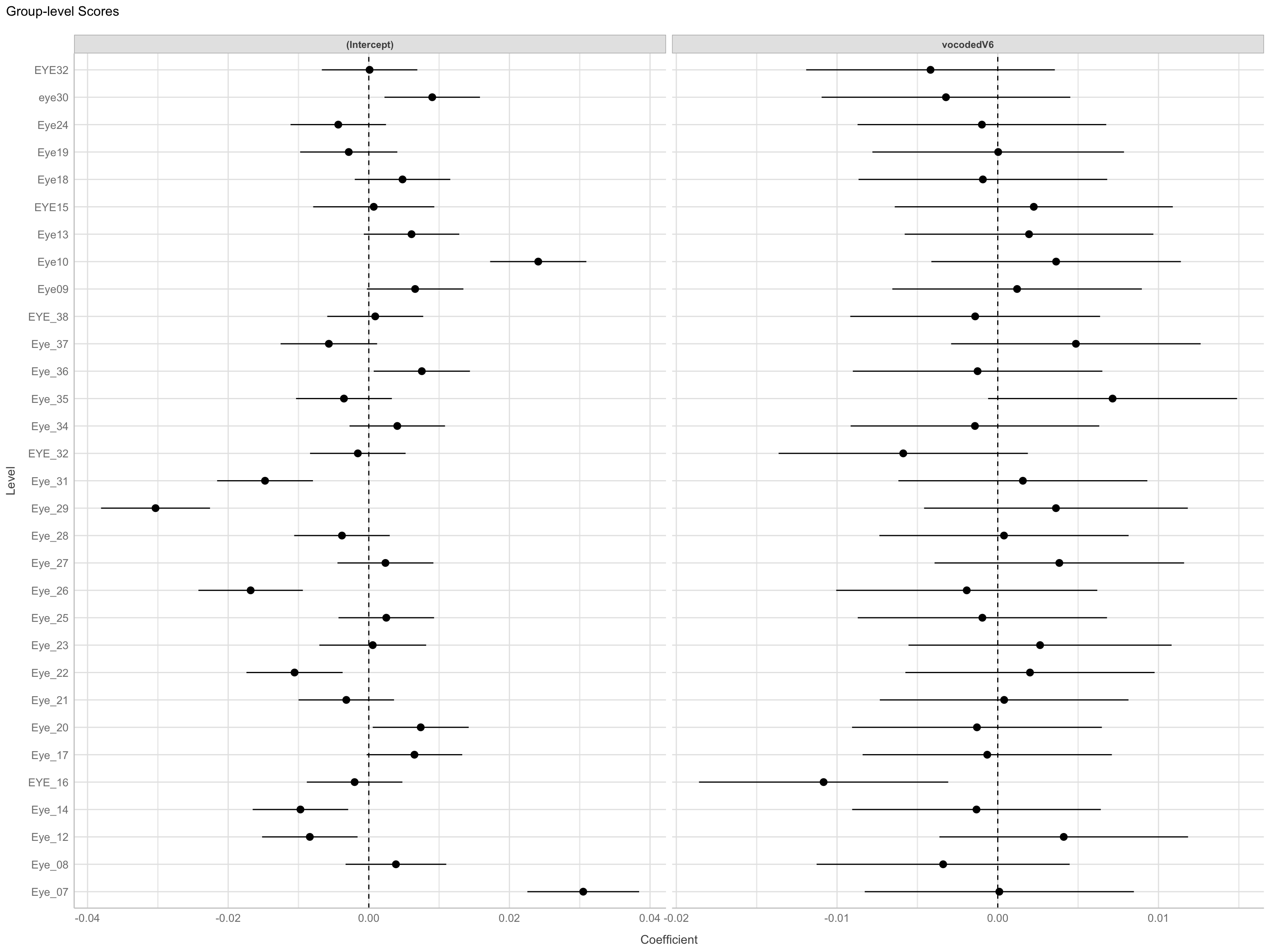
Model comparisons

Can compare models using anova function or test_likelihoodratio from easystats
- Will be refit using ML if interested in fixed effects

# you try

AIC/BIC

LRT requires nested models

AIC

AIC:

\[ D + 2p \]

where d = deviance and p = # of parameters in model
Can compare AICs¹:

\[ \Delta_i = AIC_{i} - AIC_{min} \]
Less than 2: More parsimonious model is preferred
Between 4 and 7: some evidence for lower AIC model
Greater than 10,: strong evidence for lower AIC

BIC

BIC:

\[ D + ln(n)*p \]

where d = deviance, p = # of parameters in model, n = sample size
Change in BIC:
- \(\Delta{BIC}\) <= 2 (No difference)
- \(\Delta{BIC}\) > 3 (evidence for smaller BIC model)

AIC/BIC

performance::model_performance(max_model) %>% # easystats
  kable()

AIC	AICc	BIC	R2_conditional	R2_marginal	ICC	RMSE	Sigma
-19801.66	-19801.65	-19761.87	0.0773469	0.0013442	0.076105	0.0407697	0.0409264

Hypothesis testing

Multiple options
1. t/F tests with approximate degrees of freedom (Kenward-Rogers or Satterwaithe)
2. Parametric bootstrap
3. Likelihood ratio test (LRT)
- Can be interpreted as main effects and interactions
- Use afex package to do that

Hypothesis testing - `afex`

library(afex) # load afex in 

m <- mixed(mean_pupil ~ 1 + vocoded +  (1+vocoded|subject), data =eye, method = "LRT") # fit lmer using afex

nice(m) %>%
  kable()

Effect	df	Chisq	p.value
vocoded	1	4.47 *	.034

Using `emmeans`

Get means and contrasts

library(emmeans) # get marginal means 

emmeans(max_model, specs = "vocoded") %>% 
  kable() # grabs means/SEs for each level of vocode

vocoded	emmean	SE	df	asymp.LCL	asymp.UCL
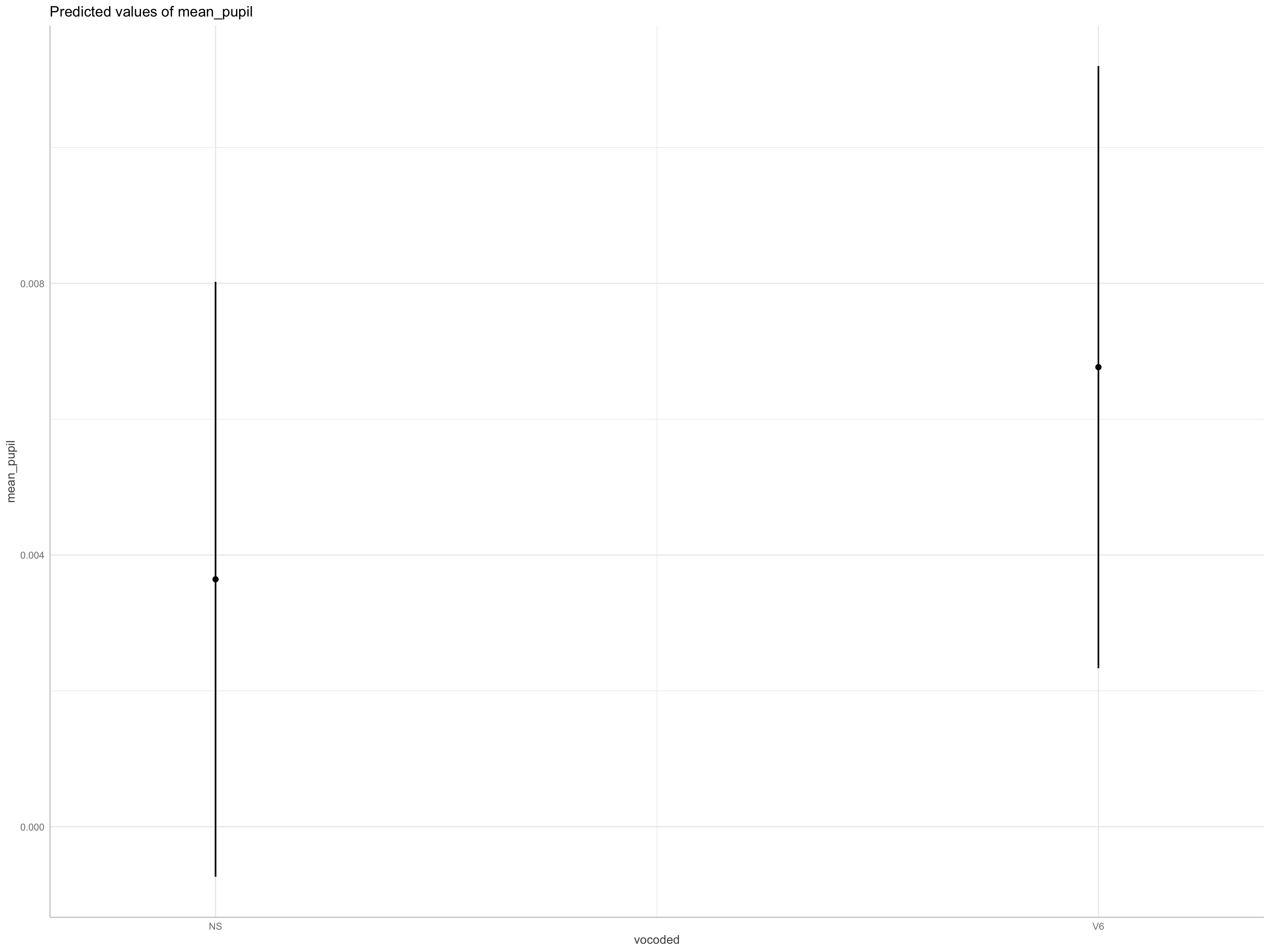
NS	0.0036427	0.0022348	Inf	-0.0007374	0.0080229
V6	0.0067668	0.0022618	Inf	0.0023337	0.0111999

pairs(emmeans(max_model, specs = "vocoded")) %>%
  confint() %>%
  kable()

contrast	estimate	SE	df	asymp.LCL	asymp.UCL
NS - V6	-0.0031241	0.0014532	Inf	-0.0059723	-0.0002759

# use this to get pariwise compairsons between levels of factors

Assumptions

Check assumptions

Linearity
Normality
- Level 1 residuals are normally distributed around zero
- Level 2 residuals are multivariate-normal with a mean of zero
Homoskedacticity
- Level 1/Level 2 predictors and residuals are homoskedastic

Collinearity
Outliers

Assumptions

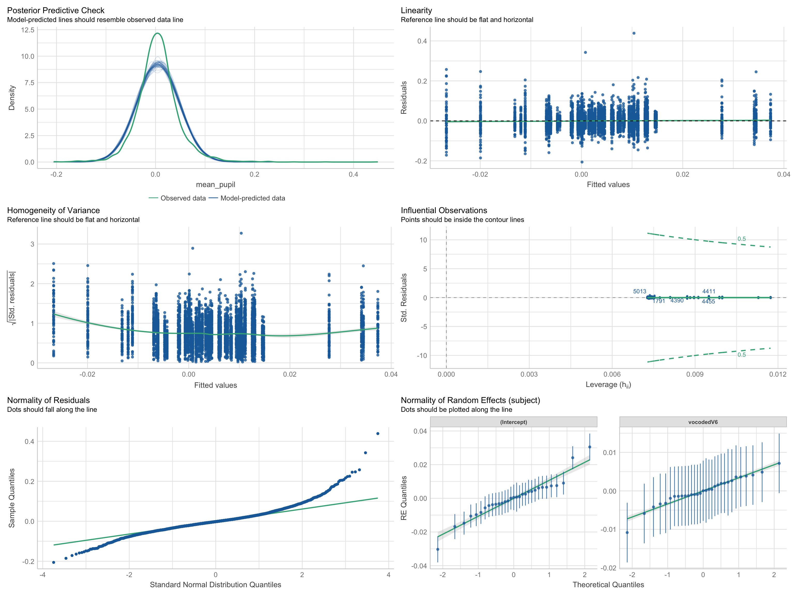
library(easystats) # performance package

check_model(max_model)

Visualization

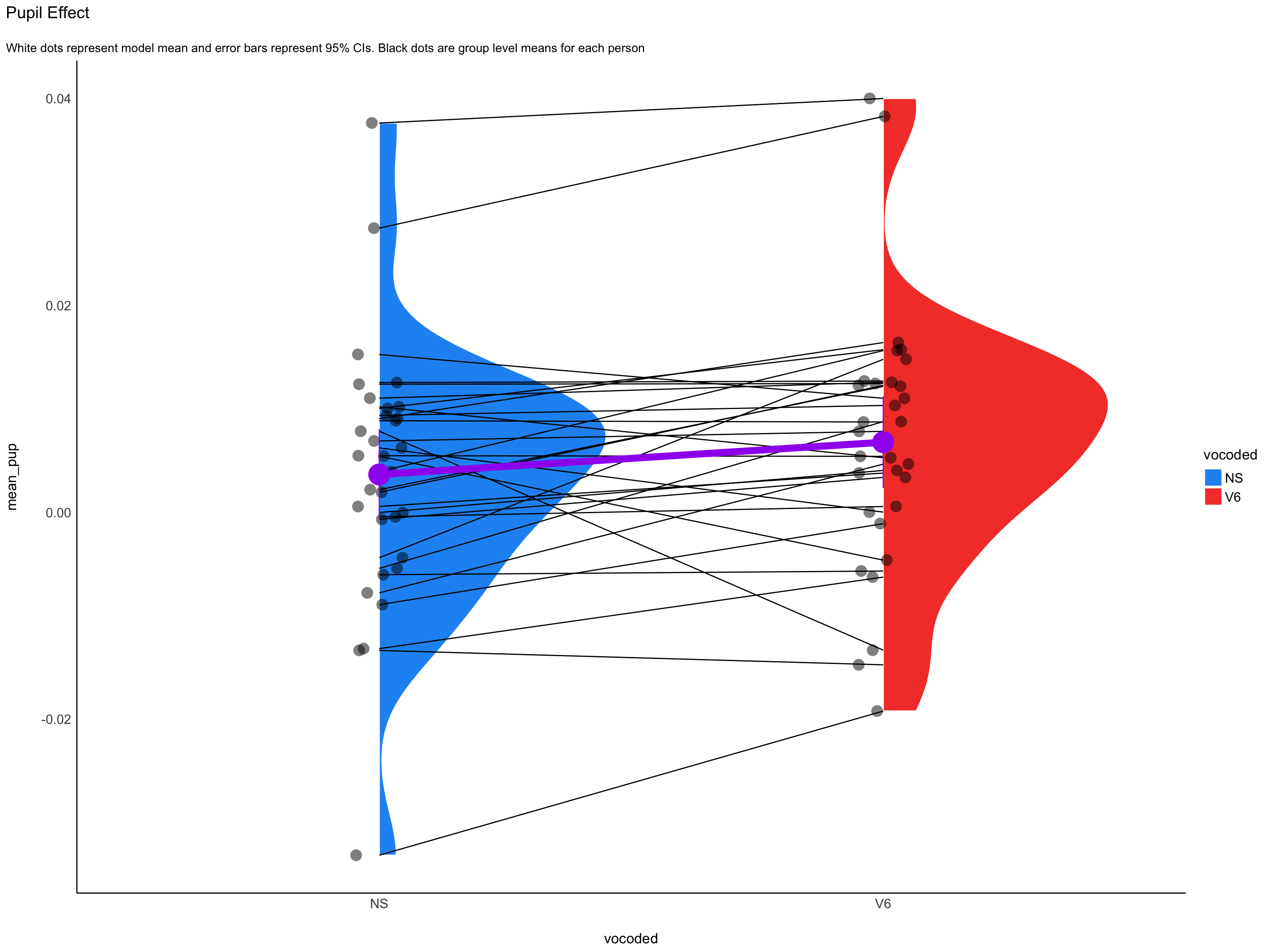
`ggeffects`

ggemmeans(max_model, terms=c("vocoded")) %>% plot()

Effect size

Report pseudo-\(R^2\) for marginal (fixed) and conditional model (full model) (Nakagawa et al. 2017)

\[ R^2_{LMM(c)} = \frac{\sigma_f^2\text{fixed} + \sigma_a^2\text{random}}{\sigma_f^2\text{fixed} + \sigma_a^2\text{random} + \sigma_e^2\text{residual}} \]

\[ R^2_{\text{LMM}(m)} = \frac{\sigma_f^2\text{fixed}}{\sigma_f^2\text{fixed} + \sigma_a^2\text{random} + \sigma_e^2\text{residual}} \]

Report semi-partial \(R^2\) for each predictor variable
- \(R^2_\beta\)
  - partR2 package in R does this for you

Effect size

#get r2 for model with performance from easystats

performance::r2(max_model)

# R2 for Mixed Models

  Conditional R2: 0.077
     Marginal R2: 0.001

# get semi-part
library(partR2)
# does not work with random slopes for some reason :/
R2_3 <- partR2(max_model,data=eye, 
  partvars = c("vocoded"),
  R2_type = "marginal", nboot = 10, CI = 0.95
)

Effect size

Cohen’s \(d\) for treatment effects/categorical predictions¹

\[ d = \frac{\text{Effect}}{\sqrt{\sigma^2_\text{Intercept} + \sigma^2_\text{slope} + \sigma^2_\text{residual}}} \]

emmeans(max_model,~ vocoded) %>% 
 eff_size(.,sigma=.04, edf=30) # need to calcuate sigma and add dfs

 contrast effect.size     SE  df asymp.LCL asymp.UCL
 NS - V6      -0.0781 0.0377 Inf    -0.152  -0.00421

sigma used for effect sizes: 0.04 
Degrees-of-freedom method: inherited from asymptotic when re-gridding 
Confidence level used: 0.95

Reporting Results

Describing a MLM analysis - Structure

What was the nested data structure (e.g., how many levels; what were the units at each level?)

• How many units were in each level, on average?

• What was the range of the number of lower-level units in each group/cluster?

Describing a MLM analysis - Model

What equation can best represent your model?
What estimation method was used (e.g., ML, REML)?
If there were convergence issues, how was this addressed?
What software (and version) was used (when using R, what packages as well)?

If degrees of freedom were used, what kind?
What type of models were estimated (i.e., unconditional, random intercept, random slope, max)?
What variables were centered and what kind of centering was used?
What model assumptions were checked and what were the results?

Describing a MLM analysis - Results

What was the ICC of the outcome variable?
Are fixed effects and variance components reported?
What inferential statistics were used (e.g., t-statistics, LRTs)?
How precise were the results (report the standard errors and/or confidence intervals)?

Were model comparisons performed (e.g., AIC, BIC, if using an LRT,report the χ2, degrees of freedom, and p value)?
Were effect sizes reported for overall model and individual predictors (e.g., Cohen’s d, \(R^2\) )?

Write-up

report::report(max_model) # easystats report function

We fitted a linear mixed model (estimated using REML and nloptwrap optimizer) to predict mean_pupil with vocoded (formula: mean_pupil ~ vocoded). The model included vocoded as random effects (formula: ~1 + vocoded | subject). The model’s total explanatory power is weak (conditional R2 = 0.08) and the part related to the fixed effects alone (marginal R2) is of 1.34e-03. The model’s intercept, corresponding to vocoded = NS, is at 3.64e-03 (95% CI [-7.38e-04, 8.02e-03], t(5603) = 1.63, p = 0.103). Within this model:

The effect of vocoded [V6] is statistically significant and positive (beta = 3.12e-03, 95% CI [2.75e-04, 5.97e-03], t(5603) = 2.15, p = 0.032; Std. beta = 0.07, 95% CI [6.49e-03, 0.14])

Standardized parameters were obtained by fitting the model on a standardized version of the dataset. 95% Confidence Intervals (CIs) and p-values were computed using a Wald t-distribution approximation.

Table

modelsummary::modelsummary(list("max model" = max_model), output="html") # modelsummary package

	max model
(Intercept)	0.004
	(0.002)
vocodedV6	0.003
	(0.001)
SD (Intercept subject)	0.012
SD (vocodedV6 subject)	0.005
Cor (Intercept~vocodedV6 subject)	−0.195
SD (Observations)	0.041
Num.Obs.	5609
R2 Marg.	0.001
R2 Cond.	0.077
AIC	−19801.7
BIC	−19761.9
ICC	0.1
RMSE	0.04

Power

Simulation-based power analyses
- Simulate new data
  - faux (https://debruine.github.io/faux/articles/sim_mixed.html)
- Use pilot data (what I would do)
  - mixedpower(https://link.springer.com/article/10.3758/s13428-021-01546-0)
  - simr (https://besjournals.onlinelibrary.wiley.com/doi/full/10.1111/2041-210X.12504)

Multilevel Modeing (with R) Part 2

Multilevel models

Today

Packages

Today’s data

Today’s data

Data organization

Data organization

Centering

Group- vs. Grand-Mean Centering

Group- vs. Grand-Mean Centering

Centering in R

Model Estimation

Maximum Likelihood

Probability vs. Likelihood

Likelihood

Likelihood

Likelihood

Likelihood

Likelihood

Likelihood

Likelihood

Log likelihood

\(\chi^2\) distribution

Comparing nested models

Drop-In-Deviance Test

Testing deviance

Model fitting: ML or REML?

Model fitting: ML or REML

Model fitting: ML or REML?

ML or REML?

ML or REML?

Fitting and Interpreting Models

Modeling approach

Modeling approach

Modeling approach

Modeling approach

Null model (unconditional means)

Null model (unconditional means)

Calculating ICC

Maximal model: Fixed effect random intercepts (subject) and slopes (vocoded) model

Fixed effects

Degrees of freedom and p-values

Random effects/variance components

Random effects/variance components

Visualize Random Effects

Model comparisons

AIC/BIC

AIC

BIC

AIC/BIC

Hypothesis testing

Hypothesis testing - afex

Using emmeans

Assumptions

Check assumptions

Assumptions

Visualization

ggeffects

Effect size

Effect size

Effect size

Reporting Results

Describing a MLM analysis - Structure

Describing a MLM analysis - Model

Describing a MLM analysis - Results

Write-up

Table

Power

Hypothesis testing - `afex`

Using `emmeans`

`ggeffects`