Generalized Linear Madness: Binary Outcome Models/Logistic Regression

Princeton University

Jason Geller, PH.D.(he/him)

2024-02-19

Packages

library(easystats)
library(MASS)
library(arm) # residual plot
library(effectsize) 
library(tidyverse)
library(equatiomatic)
library(kableExtra)
library(broom)
library(emmeans)
library(marginaleffects)
library(modelsummary)

options(scipen = 999)

• Access the .qmd document here: https://github.com/jgeller112/PSY504-Advanced-Stats-S24/blob/main/slides/04-logistic/logisticqmd.qmd

Today

• Nuts and bolts of logistic regression

  • Binomial/Bernoulli distribution
  • Logit link
  • Log-odds, odds, probabilities
  • Likelihood

• Motivating example: Weight loss, gender, BMI

  • Modeling fitting
  • Parameter interpretation
  • Model fit and model diagnostics
  • Comparing models
  • Visualizing
  • Reporting

Linear model

• Everything so far has included a continuous outcome

• Model \(y\) as a linear function of predictors

\[ Y_i = b_0 + b_1*x + e_i\]

\[Y \sim~Normal(\mu, \sigma)\]

Dichotomous outcomes

The simplest kind of categorical data is each case is binary

• Correct/incorrect
• Pass/fail
• Choose/Don’t choose
• Support/Not support
• Relapse/Not relapse

Note

We usually code these as 0s and 1s and model the probability of 1 occurring

Bye bye linear model

• Linear models are not appropriate for this type of data

  • Makes impossible predictions (values not between 0, 1)

  • Non-normality of residuals

    • \(\hat{p}\) or (1-\(\hat{p}\))

  • Heteroskedasticity

    • Variance is influenced by \(\hat{p}\)

Generalized linear model

Regression models with non-normal response likelihoods

\[\begin{align*} Y_i & \sim \mathrm{Dist}(\mu_i, \tau) \\ g(\mu_i) & = \eta_i \\ \eta_i & = \beta_0 + \beta_1 X_{1i} + \beta_2 X_{2i} + \ldots \end{align*}\]Where:

• \(y\) is referenced with \(\mu\)

• \(g\) is link function (in logistic regression we use logit link)

What distribution do we use to model this process?

• We assume that there is some probability p of responding correctly (or selecting what is coded as 1)

• We don’t know this probability, so we want to use the data to estimate it

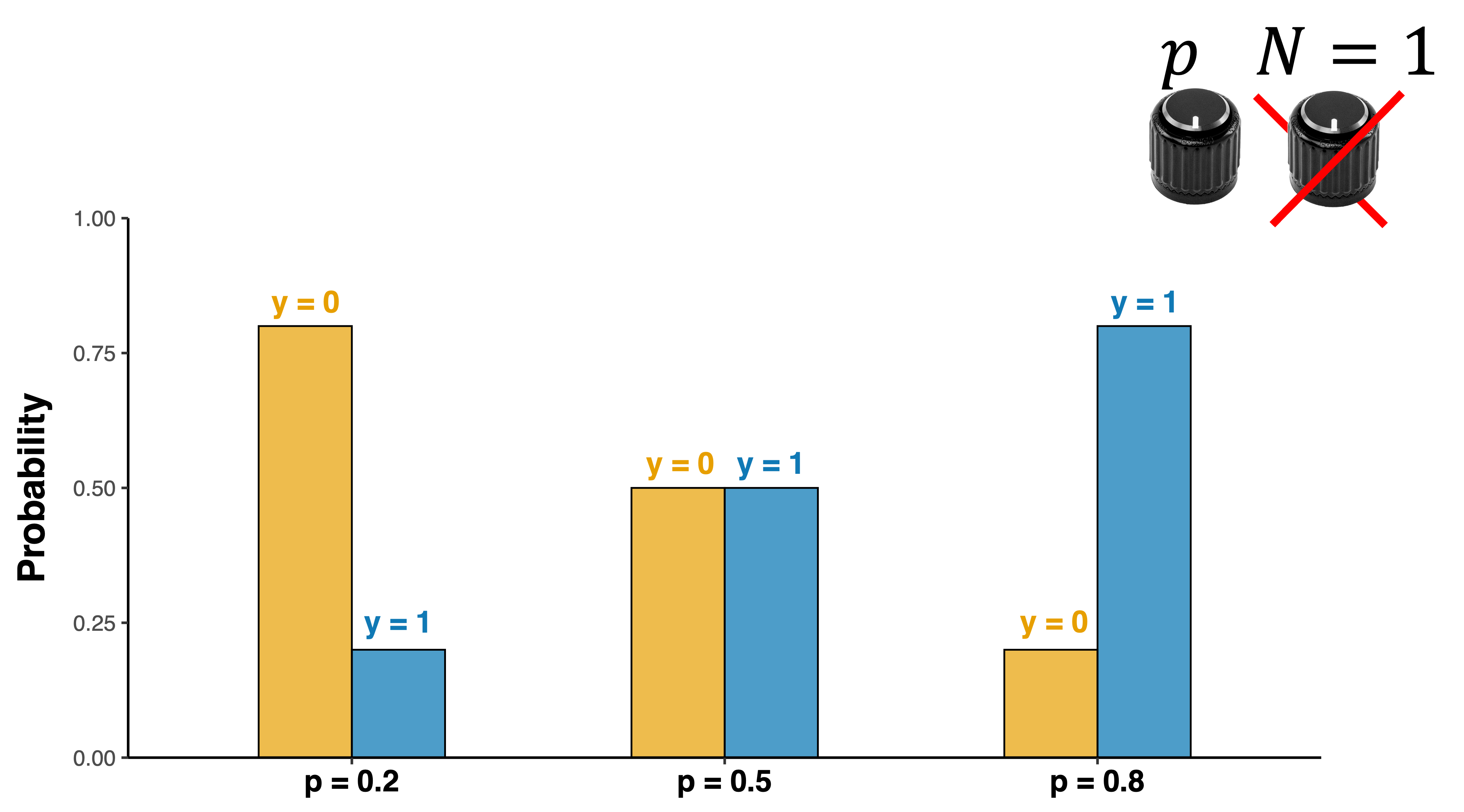
Bernoulli distribution

Distribution of a single, discrete binary outcome \[y\sim Bernoulli(p)\]

• A Bernoulli distribution generates a 1 (“success”) with probability p

• And a 0 (“failure”) with probability 1−p=q

  • \(\mu\) = E(X)=p
  • \(\sigma^2(X)=p(1-p)\)

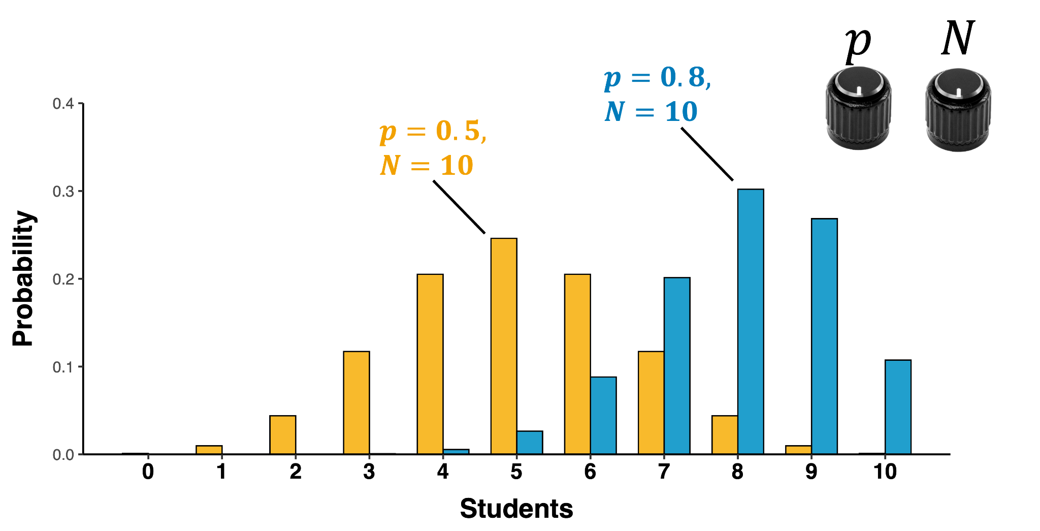
Binomial distribution

Distribution of discrete counts of independent outcomes over a certain set of trials

\[y\sim binomial(N,p)\]

• N = number of trials

• p = probability of “y = 1”
  • \(\mu\) = E(X)=np$
  • \(\sigma^2(X)=np(1-p)\)
  • \(\sigma(X)\)=\(\sqrt{np(1-p)}\)

Fitting a logistic regression in R

• In R we use the glm function as opposed to lm

  • Bernoulli
  • Binomial

  library(fivethirtyeight)
  bechdel=fivethirtyeight::bechdel
  
  #fit <- glm(
   # data = bechdel,
   # family = binomial(link="logit"),
   # binary  ~ 1 + budget_2013)
  
  bechdel %>% dplyr::select(title, binary) %>% head() %>% kable()

  title	binary
  21 & Over	FAIL
  Dredd 3D	PASS
  12 Years a Slave	FAIL
  2 Guns	FAIL
  42	FAIL
  47 Ronin	FAIL

  # one row with total # 1s and 0s instead of multiple rows 
  
  df=glm(cbind(Deaths, N-Deaths)~Species, family=binomial, data=MASS::snails)
  
  MASS::snails %>% dplyr::select(Deaths, N) %>% head() %>% kable()

  Deaths	N
  0	20
  0	20
  0	20
  0	20
  0	20
  0	20

Logit link

• The logit link transforms a linear model in the log-odds metric:

\[\begin{equation*} \log\left(\frac{p}{1 - p}\right)=b_0+b_1X \end{equation*}\]

• To a non-linear model in the probability metric:

\[\begin{equation*} p(logit)=\frac{e^{logit}}{1+e^{logit}} \end{equation*}=\frac{exp(logit)}{1+exp(logit)}\]

Logit link

• Step 1

  • Transform probability into odds

    • The “odds” of an event are just the probability it happens divided by the probability it does not happen

\[\textrm{Odds} = \frac{\# \textrm{successes}}{\# \textrm{failures}}= \frac{\# \textrm{successes}/n}{\# \textrm{failures}/n}= \frac{p}{1-p}\]

Logit Link

• Step 2

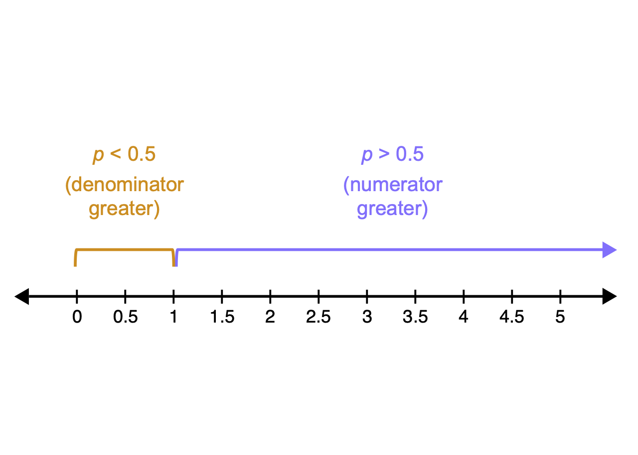
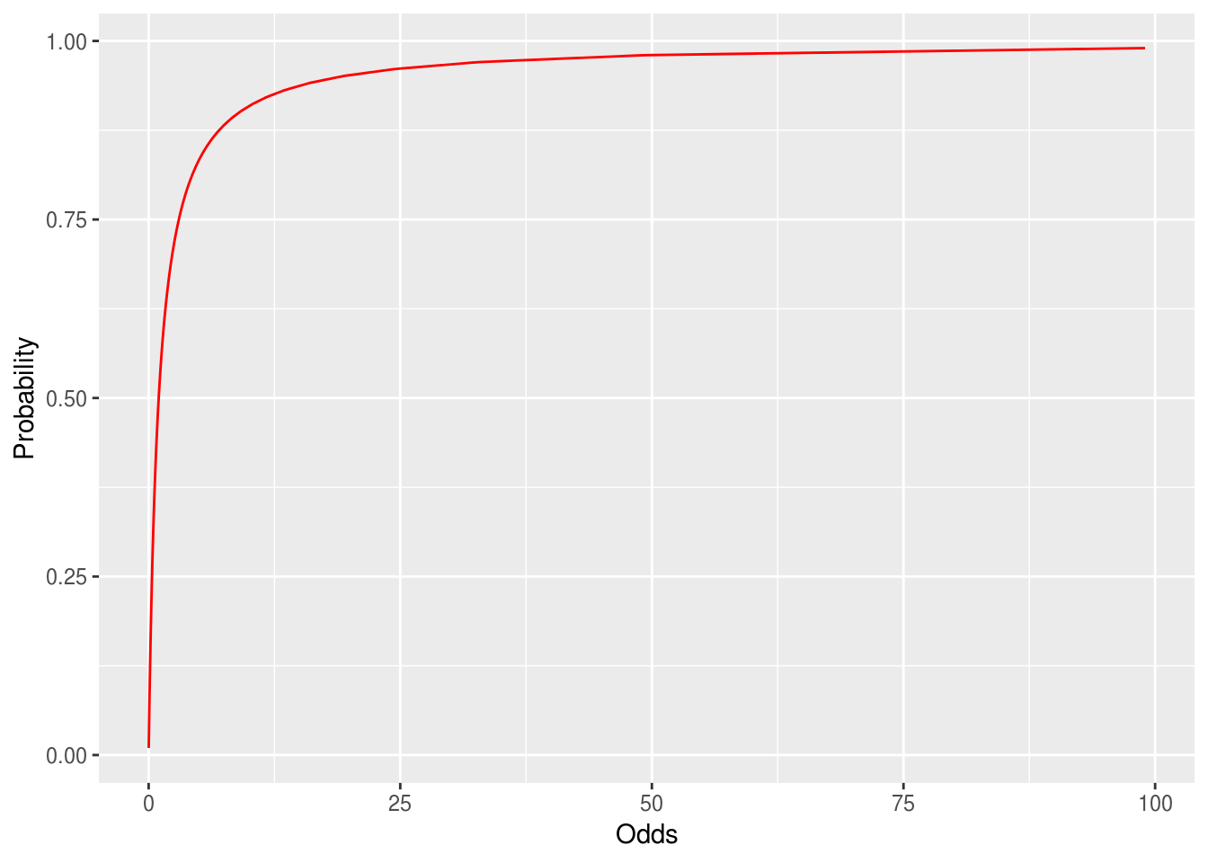
  • When we convert a probability to odds, odds always > 0

    • Asymmetric

    • Curvy

      • Problematic for linear model

  • Solution: take log of the odds

  \[logit = log(\frac{p}{1-p})\]

Logit link

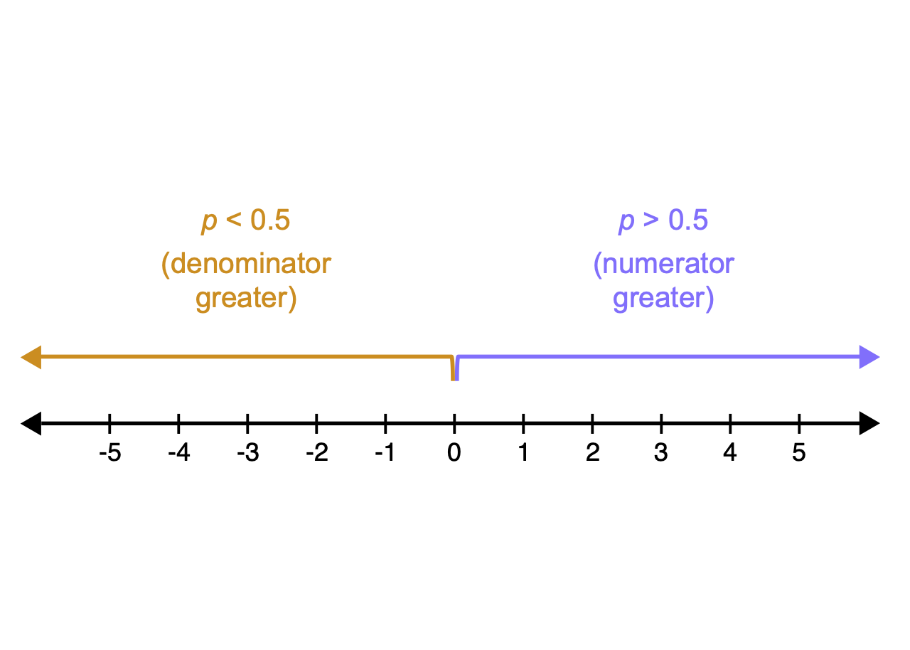
• This log odds conversion has a nice property

  • It converts odds of less than one to negative numbers, because the log of a number between 0 and 1 is always negative

    • Our data is now linear!

    • and symmetric

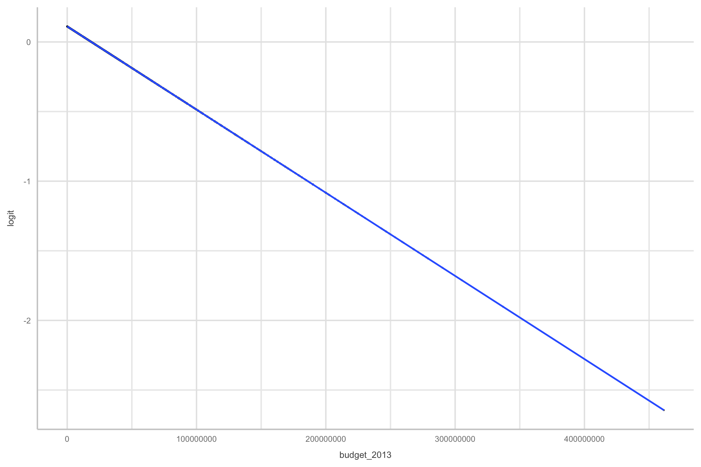
However…

• We need a function that scrunches the output of the linear predictor into a range appropriate for this parameter

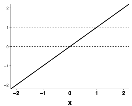
Squiggles

• We need a function that scrunches the output of the linear predictor into a range appropriate for this parameter

• A squiggle (logistic or Sigmoid curve) to the rescue!

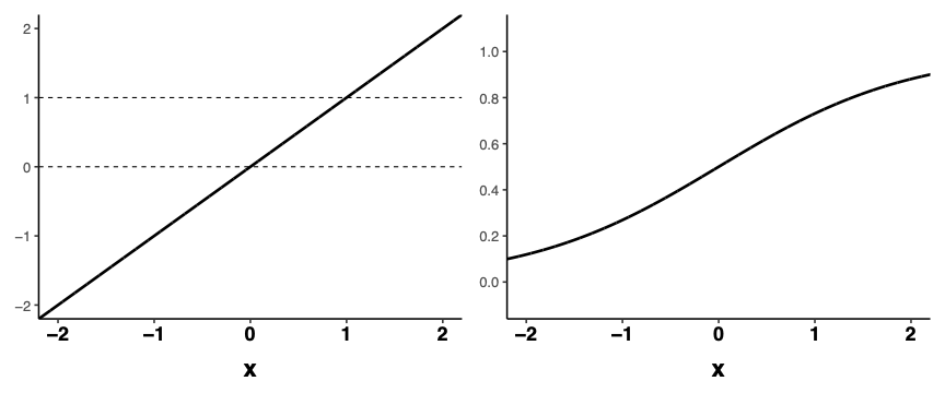
Logistic transform

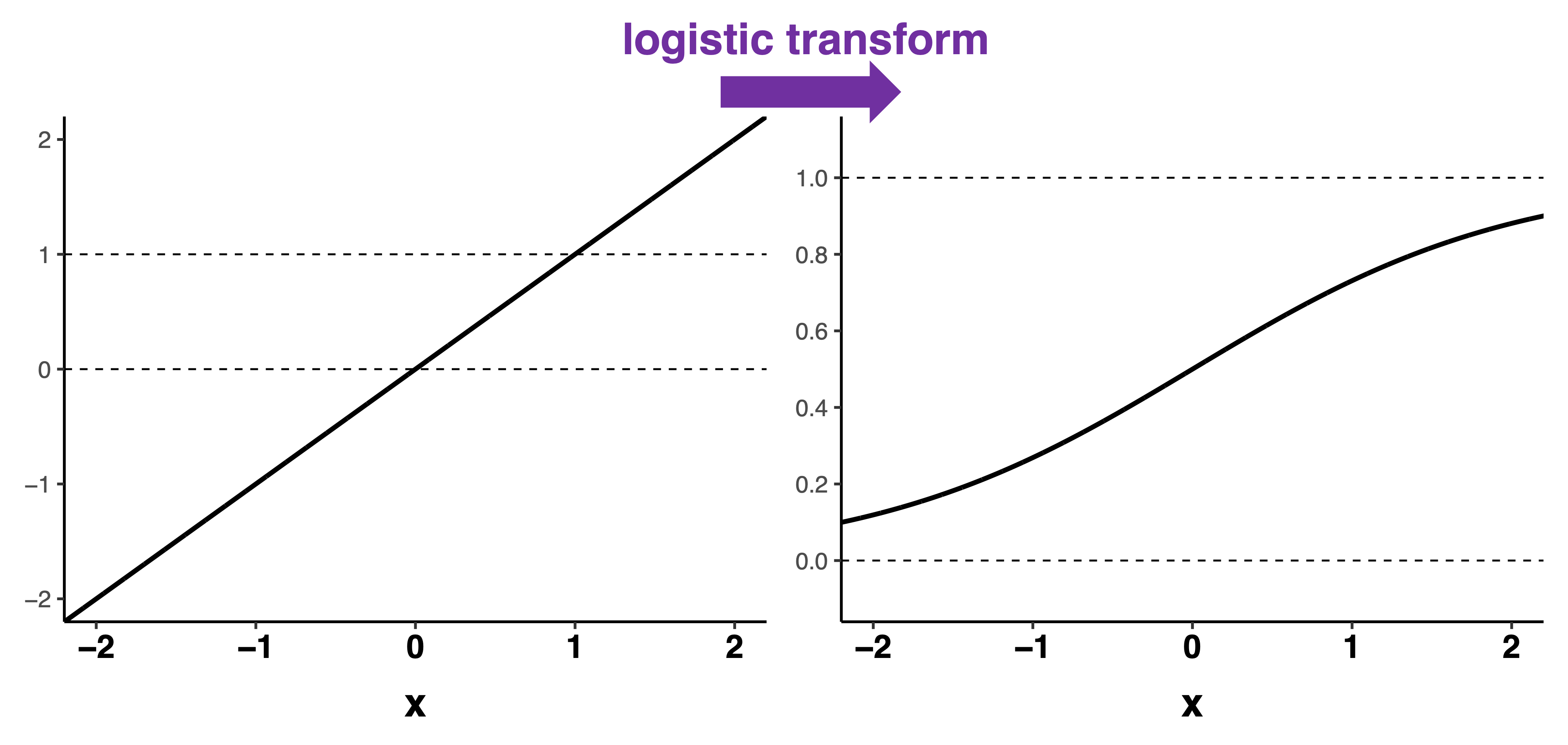
\[p(logit)=\frac{e^{logit}}{1+e^{{logit}}}\]

Slope and intercept parameters

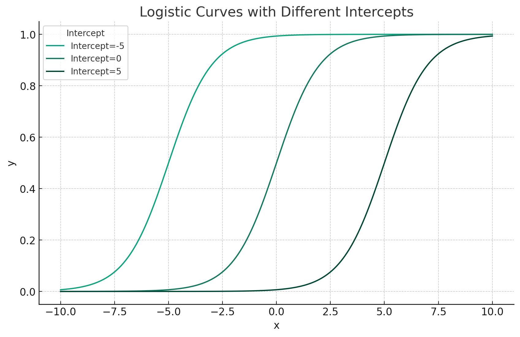
• Intercept moves curve left or right

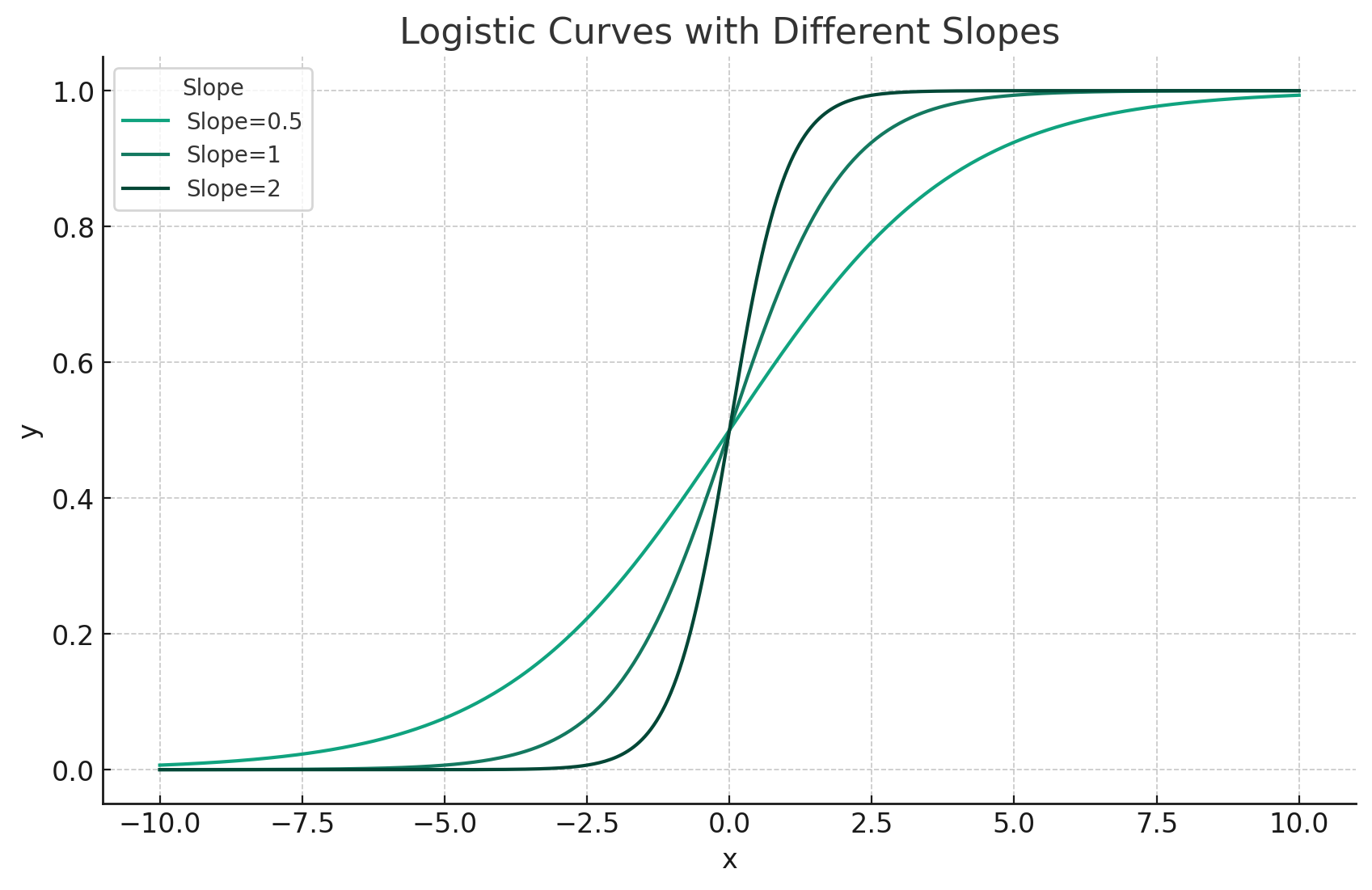
• Slope determines the steepness of the curve

All together

Andrew Heiss

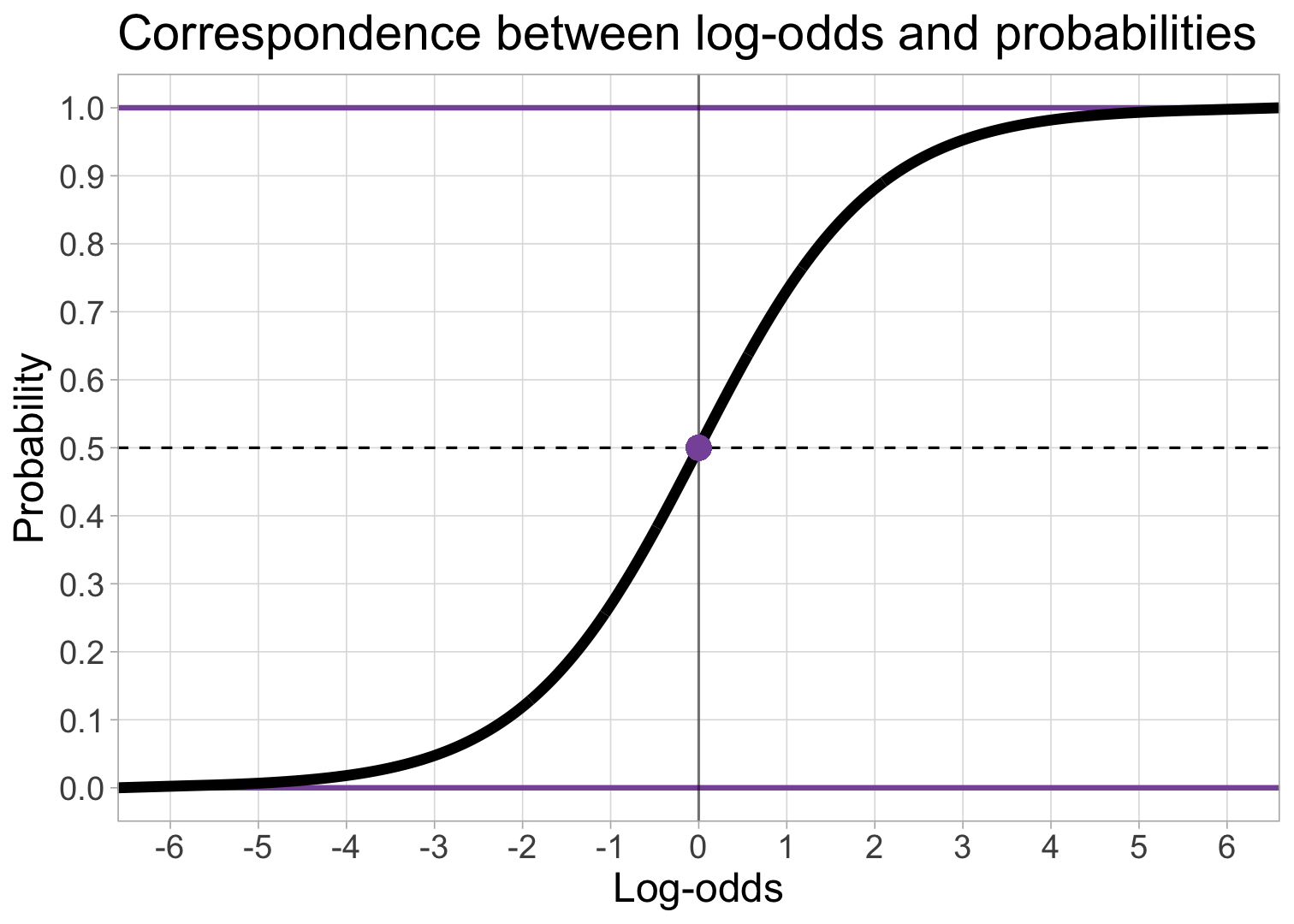
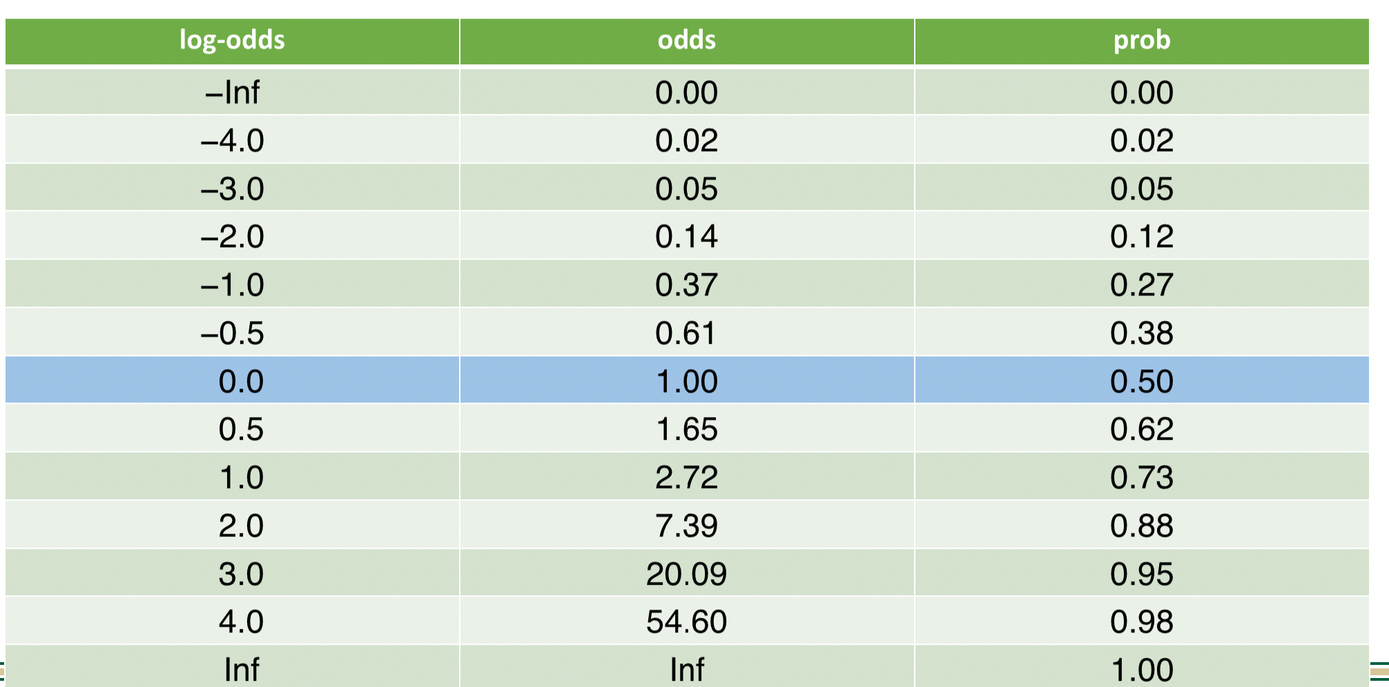
Probabilities, Odds, and Log Odds

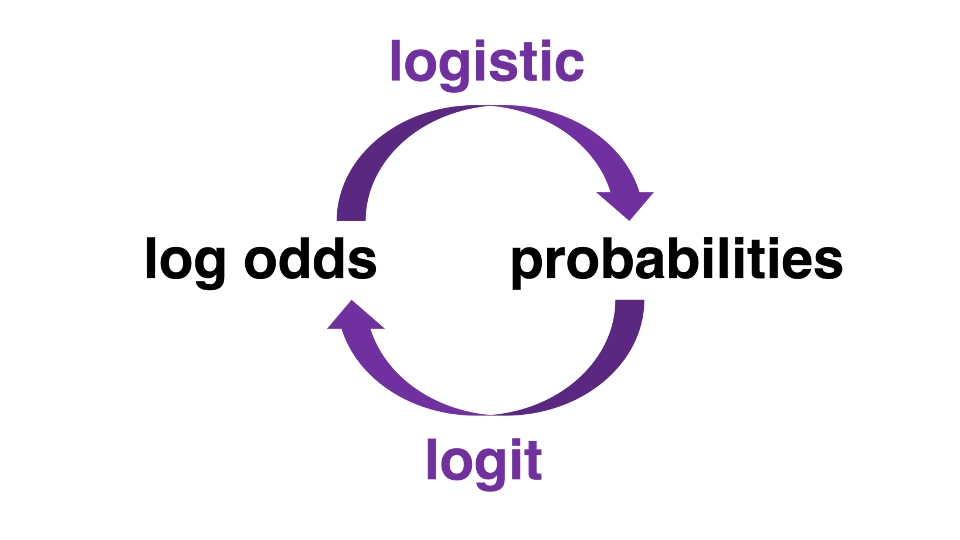
Probabilities, Odds, and Log Odds

• From probabilities to log-odds

qlogis(.3)

[1] -0.8472979

• From log-odds to probabilities

plogis(-1)

[1] 0.2689414

Probabilities, Odds, and Log Odds

Best fitting squiggle

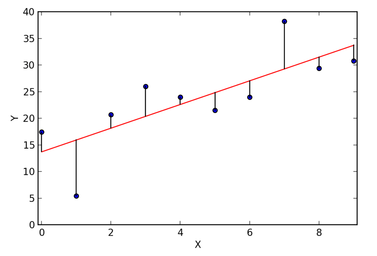
• In standard linear regression we use least squares to find the best fitting line

Maximum likelihood estimation

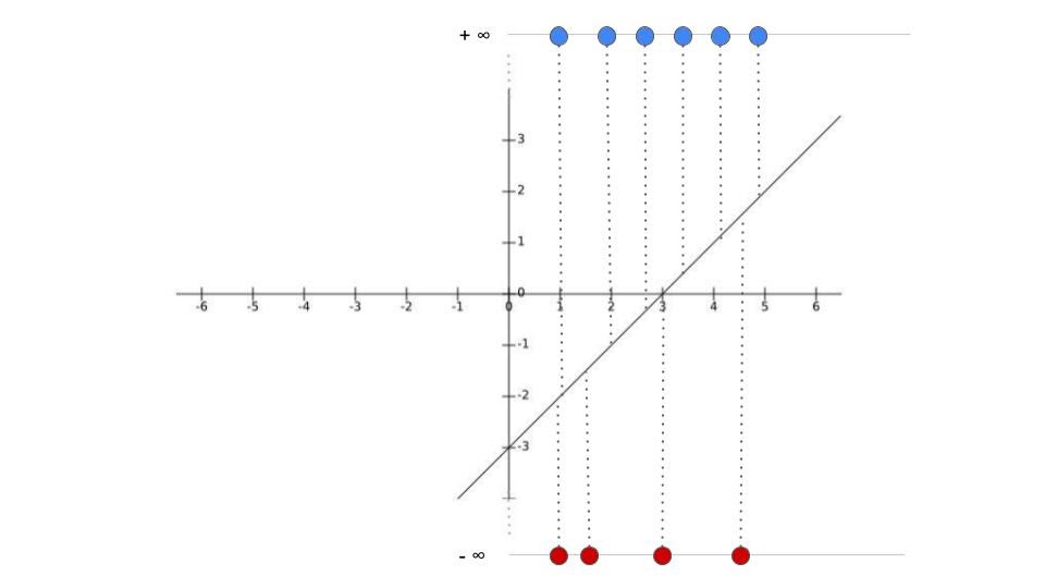
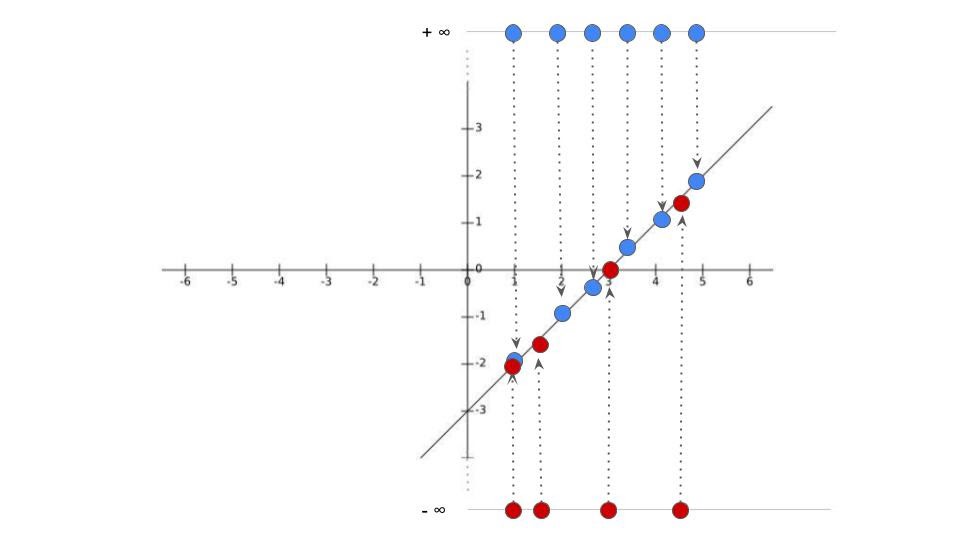
• We need find where points lie on line and get corresponding logits

ML: Logistic Regression

• Plot them as a function of probability

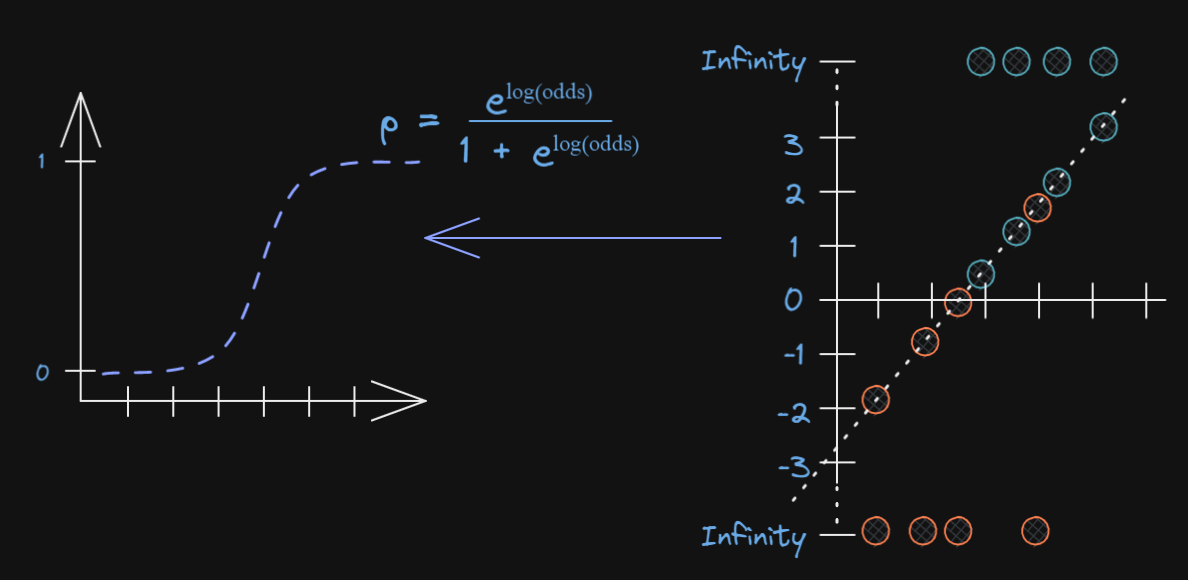
Now what?

• We keep rotating the log odds(line) and projecting data on to it and transforming into probabilities

  • Until we find maximum likelihood!

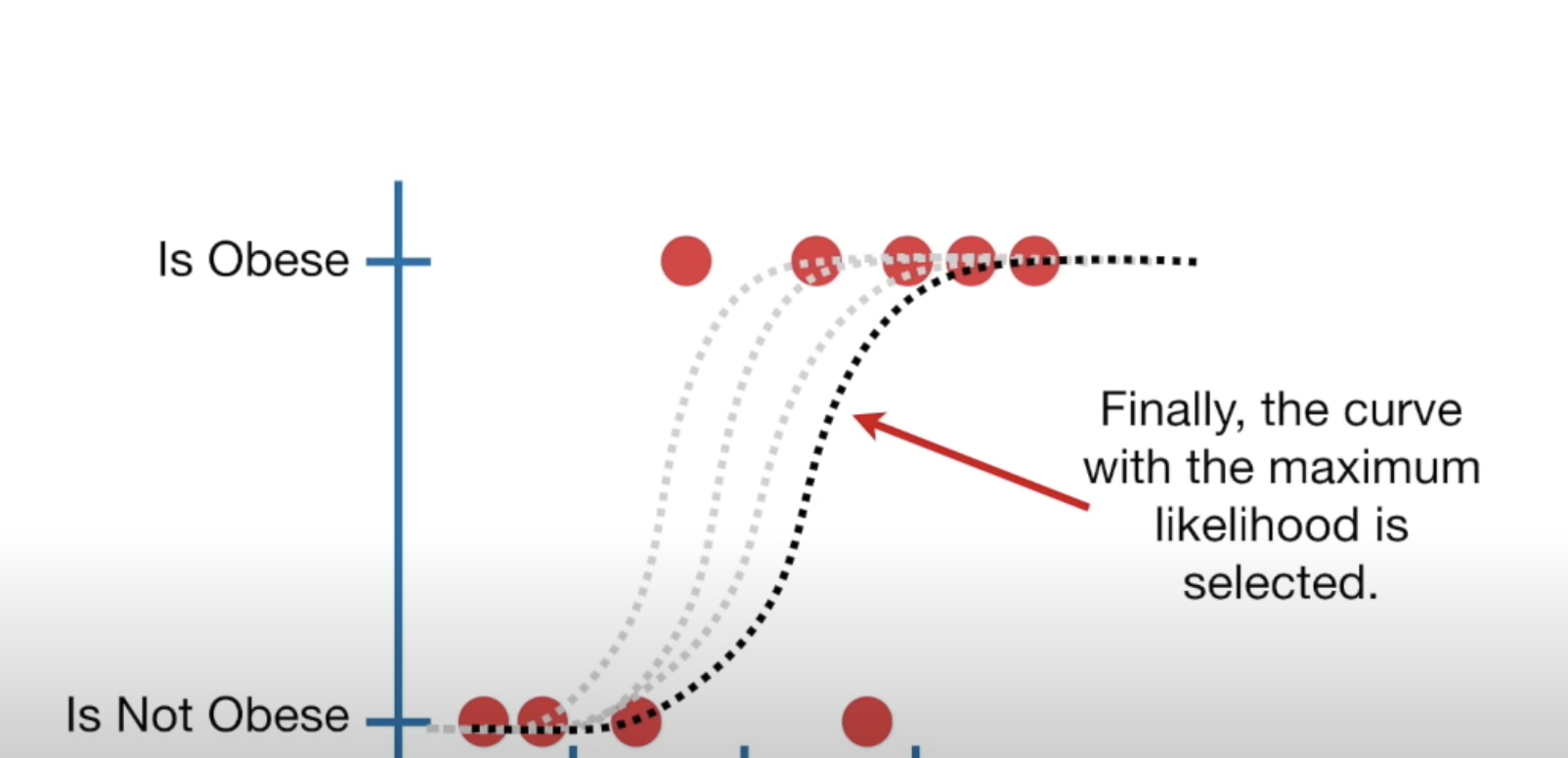
Case Study: Losing Weight

• These data are a sample of 500 teens from data collected in 2009 through the U.S. Youth Risk Behavior Surveillance System (YRBSS)

• Are the odds that young females report trying to lose weight greater than the odds that males do? Is increasing BMI associated with an interest in losing weight, regardless of sex?

Trying to lose weight

• Selected variables:

DV: *lose.wt.01, which is coded 1 when someone indicated they were trying to lost weight and 0 when they were not trying to. This is a dichotomized version of the lose.wt factor variable.

• Our two predictor variables will be:

  • sex and its related dummy variable female
  • bmipct, which is the percentile for a given BMI for members of the same sex

Exploratory data analysis

• Here are two versions of comparing lose.wt.01 by sex

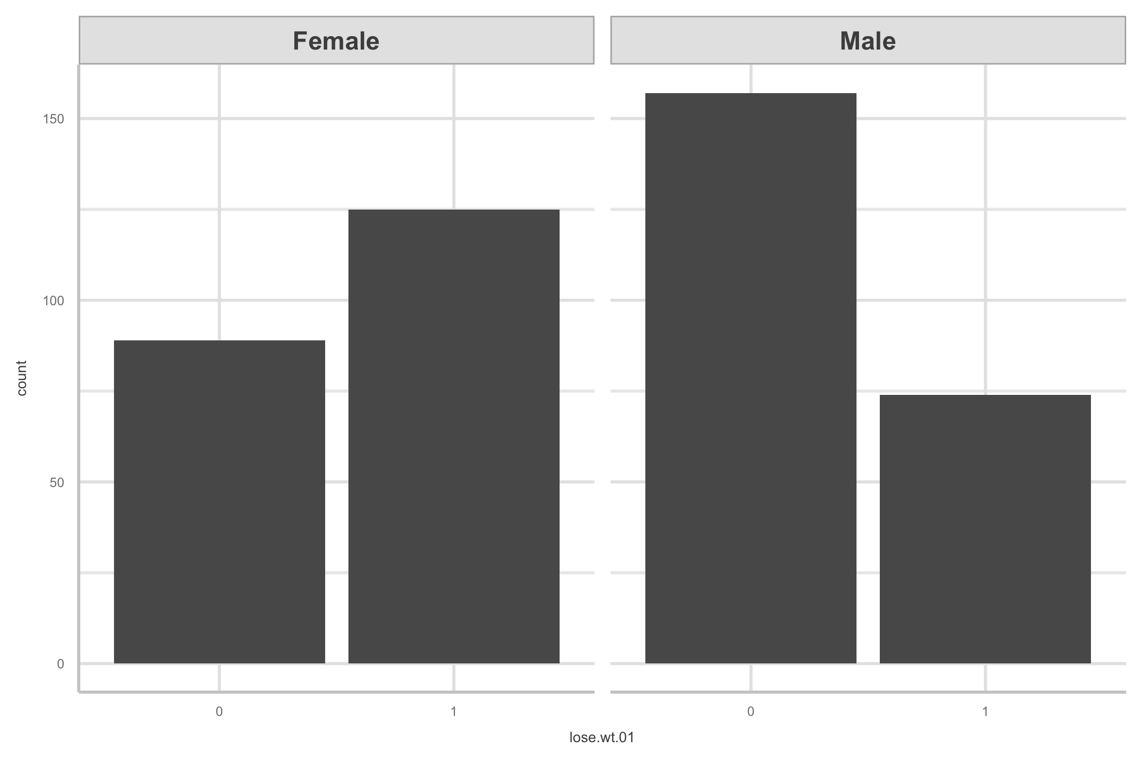
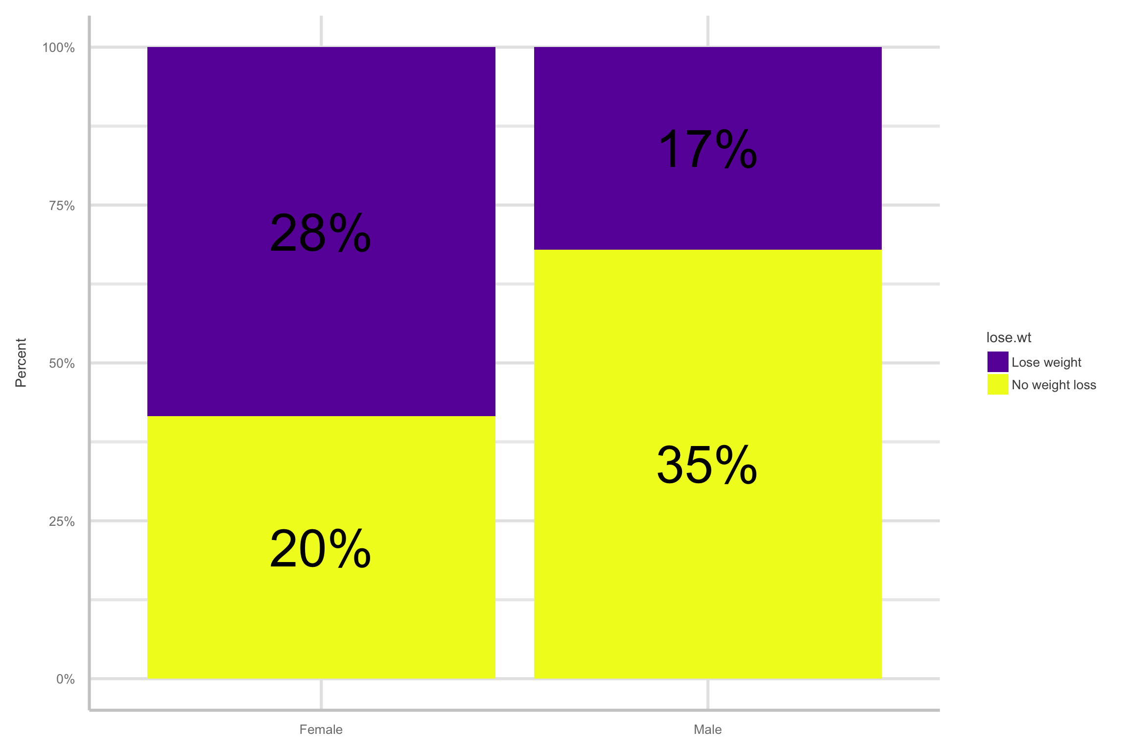
Exploratory data analysis

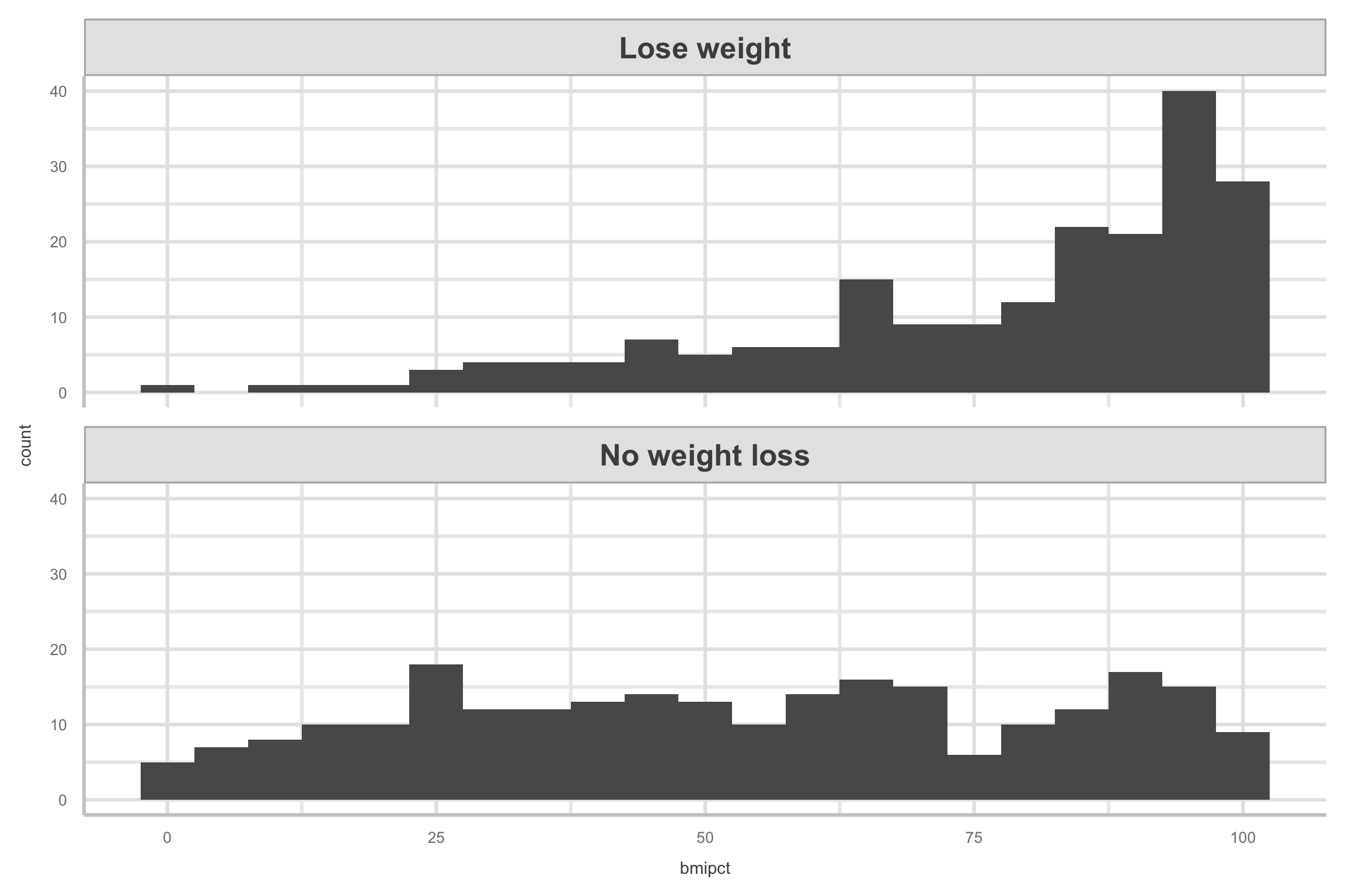
• Here are the histograms for bmipct, faceted by lose.wt.

Exploratory Data Analysis

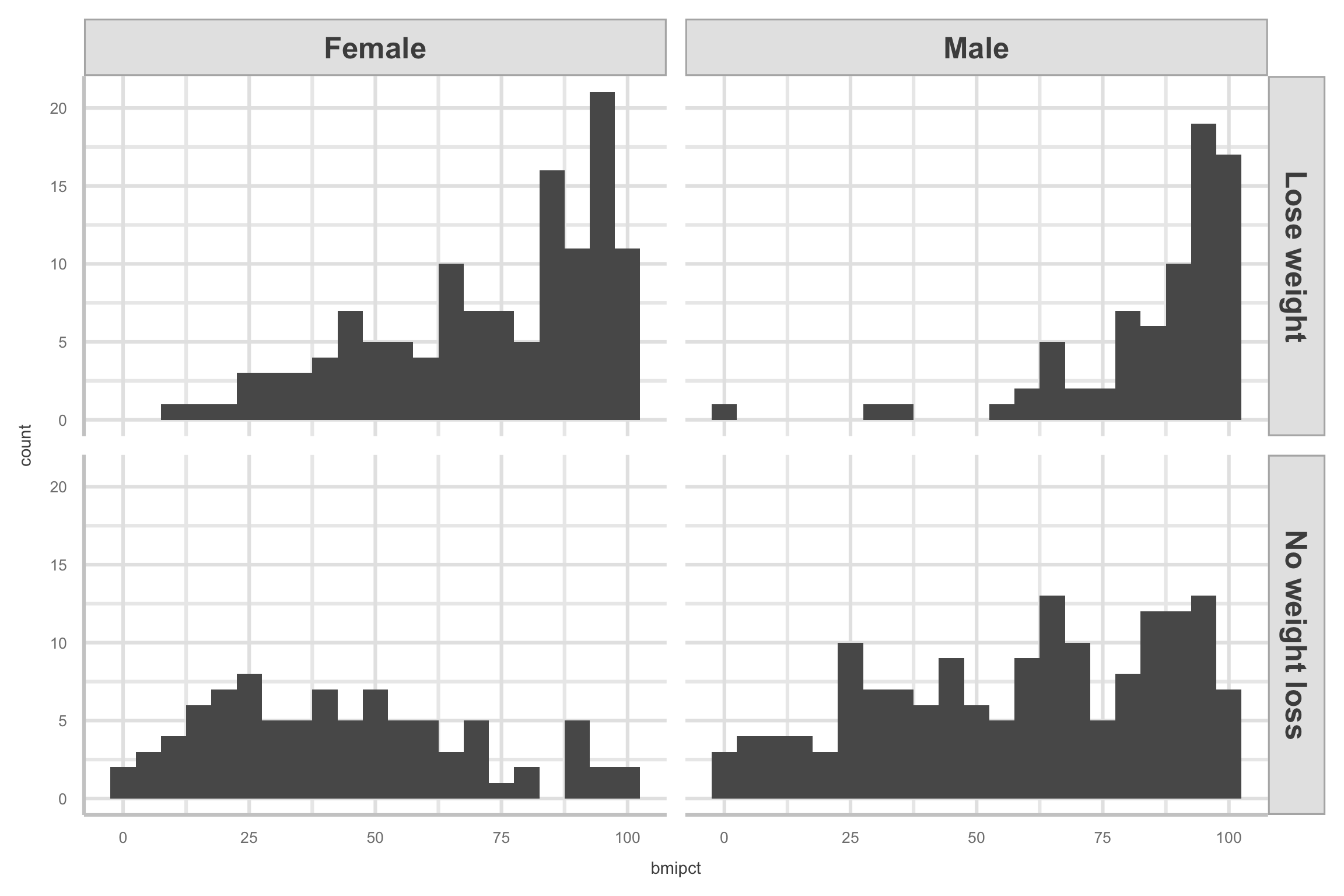
• Here are the histograms for bmipct, faceted by both lose.wt and sex

Logistic regression: Fitting model

• Let’s fit an intercept-only model

\[ \begin{align*} \text{lose.wt.01}_i & \sim \operatorname{Binomial}(n = 1, p_i)\\ \text{logit}(p_i) & = \beta_0 \end{align*} \]

Logistic Regression: Fitting Model

term	estimate	std.error	statistic	p.value
(Intercept)	-0.2120267	0.0953418	-2.22386	0.0261579

Hypothesis test for \(\beta_j\)

• Hypotheses:

  • \(H_0\): \(\beta_j\) = 0

  • \(H_a\): \(\beta_j \neq 0\)

• Test Statistic: \[\text{Wald z} = \frac{\hat{\beta}_j - 0}{SE_{\hat{\beta}_j}}\]

• CIs: \[\Large{\hat{\beta}_j \pm z^* SE_{\hat{\beta}_j}}\]

Interpreting \(b_0\)

term	estimate	std.error	statistic	p.value
(Intercept)	-0.2120267	0.0953418	-2.22386	0.0261579

• The intercept \(\beta_0\) is in the log-odds metric

  • Log-odds of Y = 1 is -0.212

• We can convert it to probability

• Thus, the overall probability of students wanting to lose weight was about .45 or 45%

Interpreting \(b_0\)

• Let’s check that with the empirical proportions

• We can actually do that transformation with the base R plogis() function

Logistic Regression

• Add our binary predictor female, which gives us the model

\[ \begin{align*} \text{lose.wt.01}_i & \sim \operatorname{Binomial}(n = 1, p_i) \\ \text{logit}(p_i) & = \beta_0 + \beta_1 \text{female}_i, \end{align*} \]

• Where female is an 0/1 dummy variable.

Interpreting intercept: \(b_0\)

• \(b_0\):

Interpreting slope: \(b_1\)

• If X is a categorical predictor

  • Then \(b_1\) is the difference in the log-odds between group X and the baseline

• Going from men to women, there is a change in the the log odds of wanting to lose weight of 1.09

Coefficient effect size: Odd’s Ratio

• We can take the exp() of the log odds and get OR

  • The odds of Y for group X (females) are expected to be exp(\(b_1\)) times the odds of Y for the baseline group

    • Greater than 1: One unit increase, the event is more likely to occur

    • Less than 1: One unit increase, the event is less likely to occur

    • Equals 1: One unit increase, the likelihood of the event does not change

  • We can describe the OR in terms of percentage increase/decrease

(OR-1) * 100  # get probability of increase/decrease

Coefficient Effect Size: Odd’s Ratio

• The odds of wanting to lose weight in females is 2.98 times the odds of wanting to lose weight in men

  • The odds of females wanting to lose weight are 198% higher than the odds of males wanting to lose weight

Predicted probabilities

• Now we can compute the probabilities for young men and women as follows

Emmeans

• Can use emmeans to get probabilities directly from model

  • Can also get odds ratios for comparisons!

  emm <- emmeans(fit2, "female", type = "response")
  emm

   female  prob     SE  df asymp.LCL asymp.UCL
        0 0.320 0.0307 Inf     0.263     0.383
        1 0.584 0.0337 Inf     0.517     0.648
  
  Confidence level used: 0.95 
  Intervals are back-transformed from the logit scale 

  # get odd ratio for comparison
  pairs(emm, reverse=TRUE)

   contrast          odds.ratio    SE  df null z.ratio p.value
   female1 / female0       2.98 0.589 Inf    1   5.520  <.0001
  
  Tests are performed on the log odds ratio scale 

Marginal effects

• We can also calculate differences in probabilities

  • Difference in probabilities is called risk difference

• Marginal effects

  • Change in probability that the outcome occurs for a 1 unit change in the predictor

    • Average marginal effect (AME)

• For categorical variables it is just probability difference between the group

#can do this with emmeans but requires more steps
library(marginaleffects) # get predicted probs
# get marginal effects
avg_comparisons(fit2, comparison = "difference") %>% 
  kable()

term	contrast	estimate	std.error	statistic	p.value	s.value	conf.low	conf.high
female	1 - 0	0.2637658	0.0455817	5.786657	0	27.05335	0.1744273	0.3531044

Logistic regression continuous

Now we add our continuous predictor bmipct, which gives us the model:

\[ \begin{align*} \text{lose.wt.01}_i & \sim \operatorname{Binomial}(n = 1, p_i) \\ \text{logit}(p_i) & = \beta_0 + \beta_1 \text{bmipct}_i, \end{align*} \]

Logistic regression continuous

term	estimate	std.error	statistic	p.value
(Intercept)	-2.5685641	0.3138083	-8.185138	0
bmipct	0.0355475	0.0042828	8.300008	0

What is the OR for \(b_1\)? How do we interpret this?

Marginal effects

• With continuous variables, obtaining the marginal effects is a bit trickier

  • Instantaneous rate of change in the predicted probability

    • Change in the predicted probability for a very small change in X

#effect is computed for each observed value in the original dataset before being averaged
avg_slopes(fit3)%>%kable()

term	estimate	std.error	statistic	p.value	s.value	conf.low	conf.high
bmipct	0.0071934	0.0005805	12.39111	0	114.7217	0.0060556	0.0083312

Tip

An increase in BMI results in 70% increase in likelihood of wanting to lose weight

Logistic Multiple Predictors

• The first will have both female and bmipct as predictors:

\[ \begin{align*} \text{lose.wt.01}_i & \sim \operatorname{Binomial}(n = 1, p_i) \\ \text{logit}(p_i) & = \beta_0 + \beta_1 \text{female}_i + \beta_2 \text{bmipct}_i. \end{align*} \]

• The second model will add an interaction term between the two predictors:

\[ \begin{align*} \text{lose.wt.01}_i & \sim \operatorname{Binomial}(n = 1, p_i) \\ \text{logit}(p_i) & = \beta_0 + \beta_1 \text{female}_i + \beta_2 \text{bmipct}_i + \beta_3 \text{female}_i \cdot \text{bmipct}_i. \end{align*} \]

Fitting both models

Model Comparisons

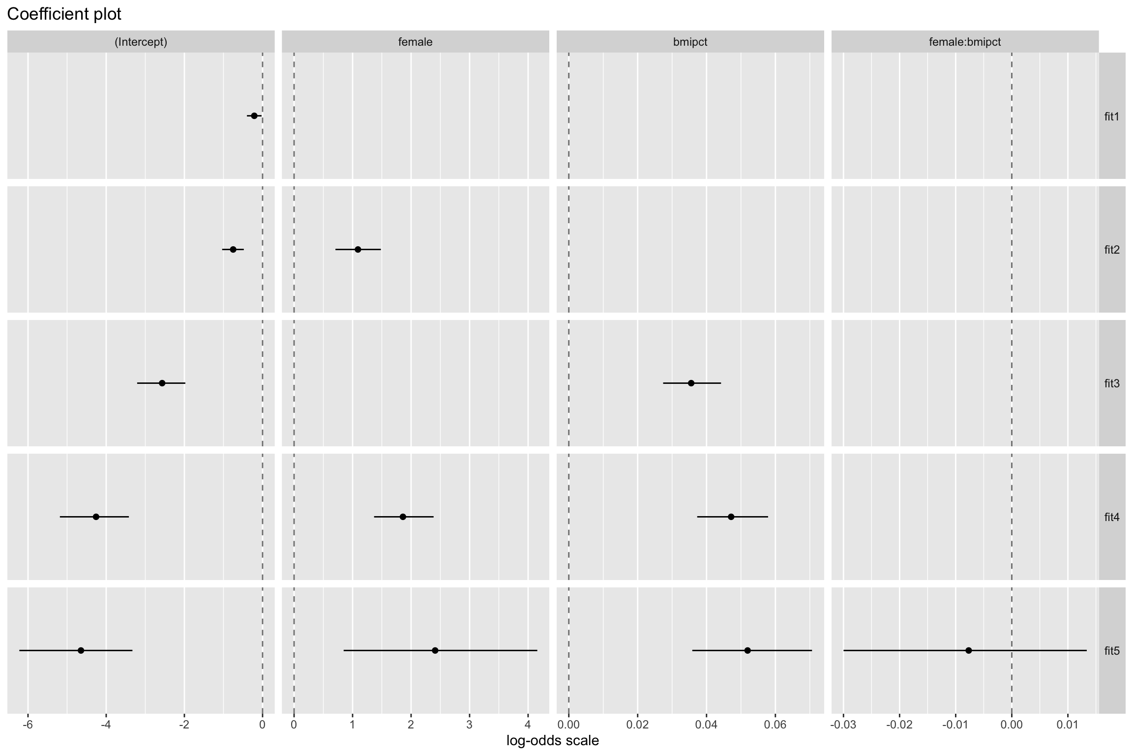
• The interaction term female:bmipct (i.e., \(\beta_3\)) would not be statistically significant

Likelihood ratio test

• Let’s compare the models by performing likelihood ratio test

test_likelihoodratio(fit4, fit5) %>% kable()

	Name	Model	df	df_diff	Chi2	p
fit4	fit4	glm	3	NA	NA	NA
fit5	fit5	glm	4	1	0.4976291	0.4805437

• When you compare model fit4 with the interaction model fit5, it appears that the interaction term does not add anything

Model Fit

• McFadden Psuedo \(R^2\)

\[R^2 = \frac{SSM}{SST} = \frac{SST-SSE}{SST}=1-\frac{SSE}{SST}\] \[R_{MF}^2 = 1-\frac{D_{\rm residual}}{D_{\rm null}}\]

#easystats function
r2_mcfadden(fit4)

# R2 for Generalized Linear Regression
       R2: 0.243
  adj. R2: 0.240

#r2_tjur
#lots others

• Not “explained variance” but ratio indicating how “good” the model fit Model Fit

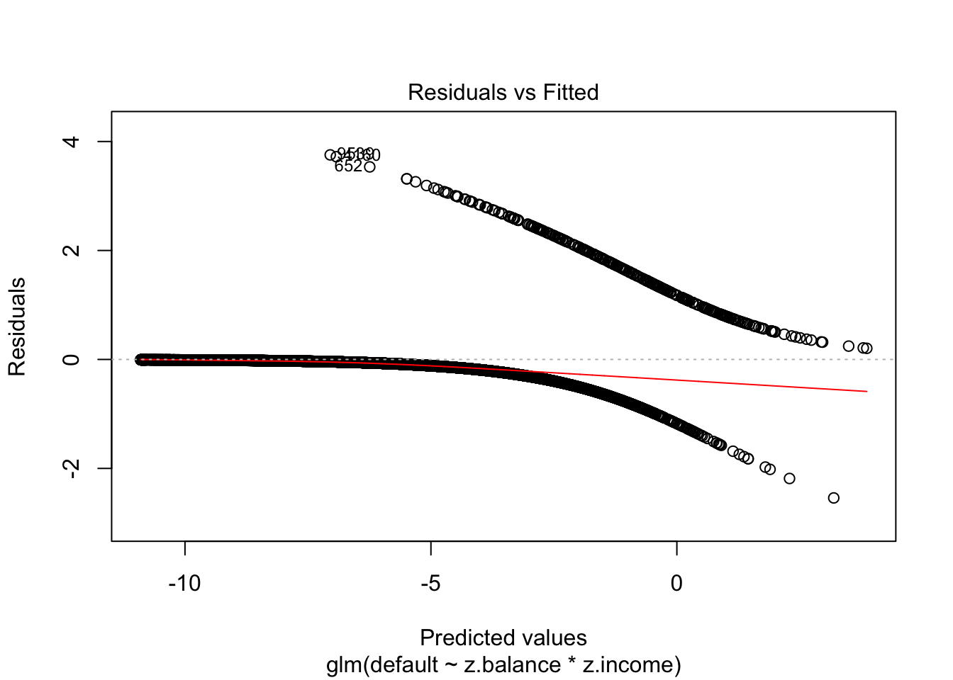
Model fit

• Plotting normal residuals are not really informative/useful

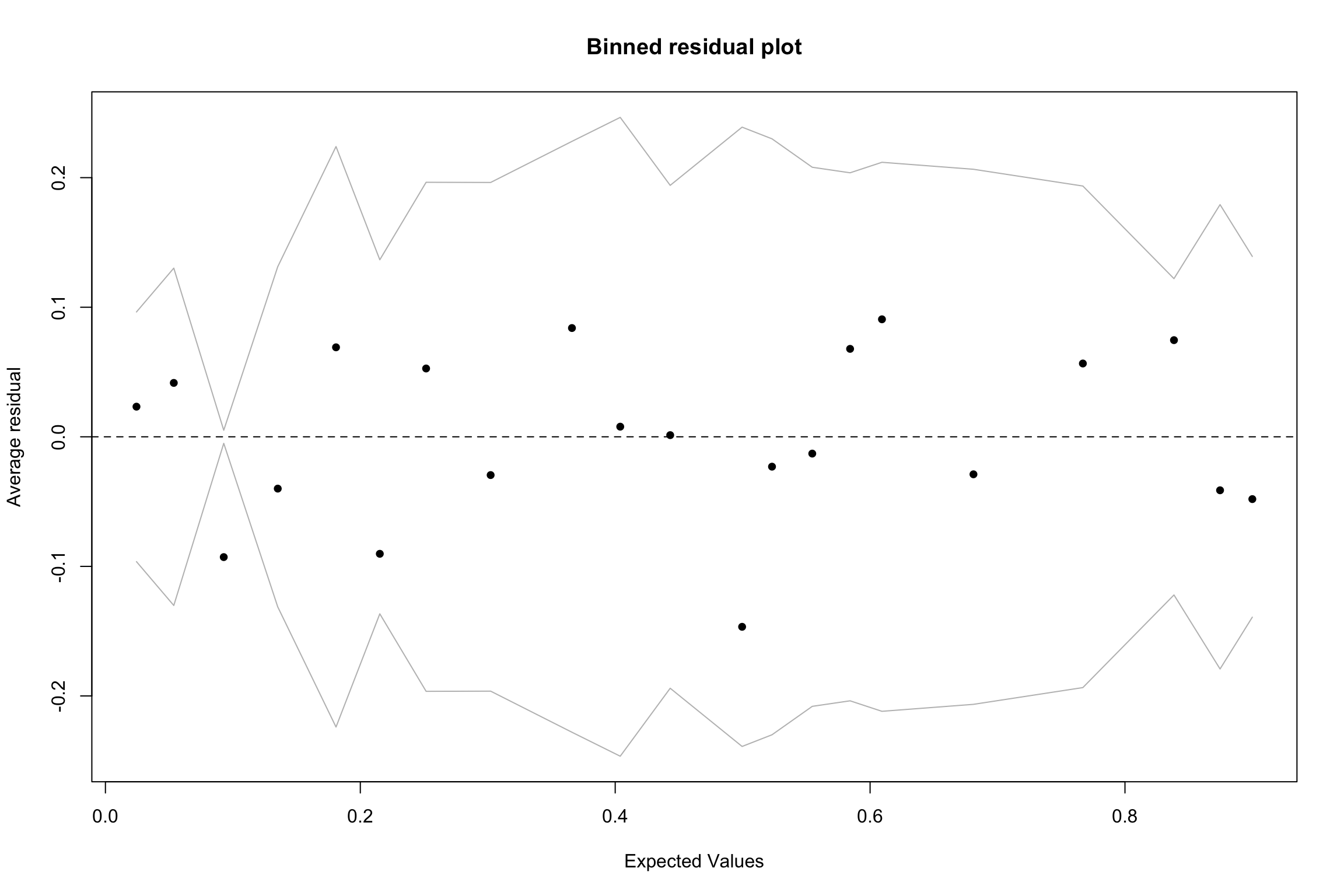
Binned residuals

• Binned residuals

  • Calculate raw residuals
  • Order observations (probabilities of DV or predictor variable)
    • Create g bins of approximate equal size \(\sqrt(n)\)
  • Calculate average residuals
  • Plot average residuals vs. average predicted probability (or predictor value)

#performance::binned_residuals()
binnedplot(fitted(fit4), residuals(fit4, type="response"))

Binned residuals

• Look for patterns

  • Nonlinear trend may be indication that squared term or log transformation is required

• If bins have average residuals with large magnitude

  • Look at averages of other predictors across bins

  • Interaction may be required

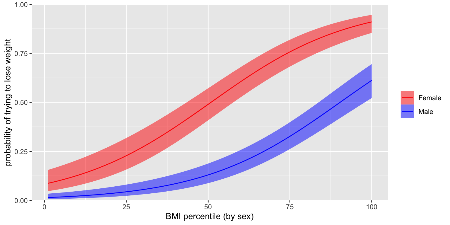
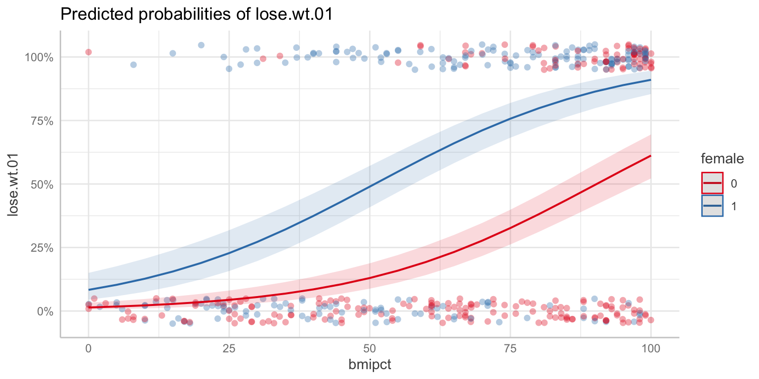
Visualizing

• ggplot
• ggeffects

library(ggeffects)
ggemmeans(fit4, terms=c("bmipct", "female")) %>%
  plot(ci = TRUE, add.data = TRUE, jitter=.05)

Assumptions

Logistic regression assumptions

• Outcome is dichotomous

• Observations are independent

• Linearity (in the log odds)

• No normality assumptions

• Homogeneity of variance

  • Variance varies with \(p\)

Logistic regression assumptions

• Can plot with easystats :)

  Note

  • Should check binned residuals of the predictor variables as well

check_model(fit4, check=c("binned_residuals", "outliers", "vif"))

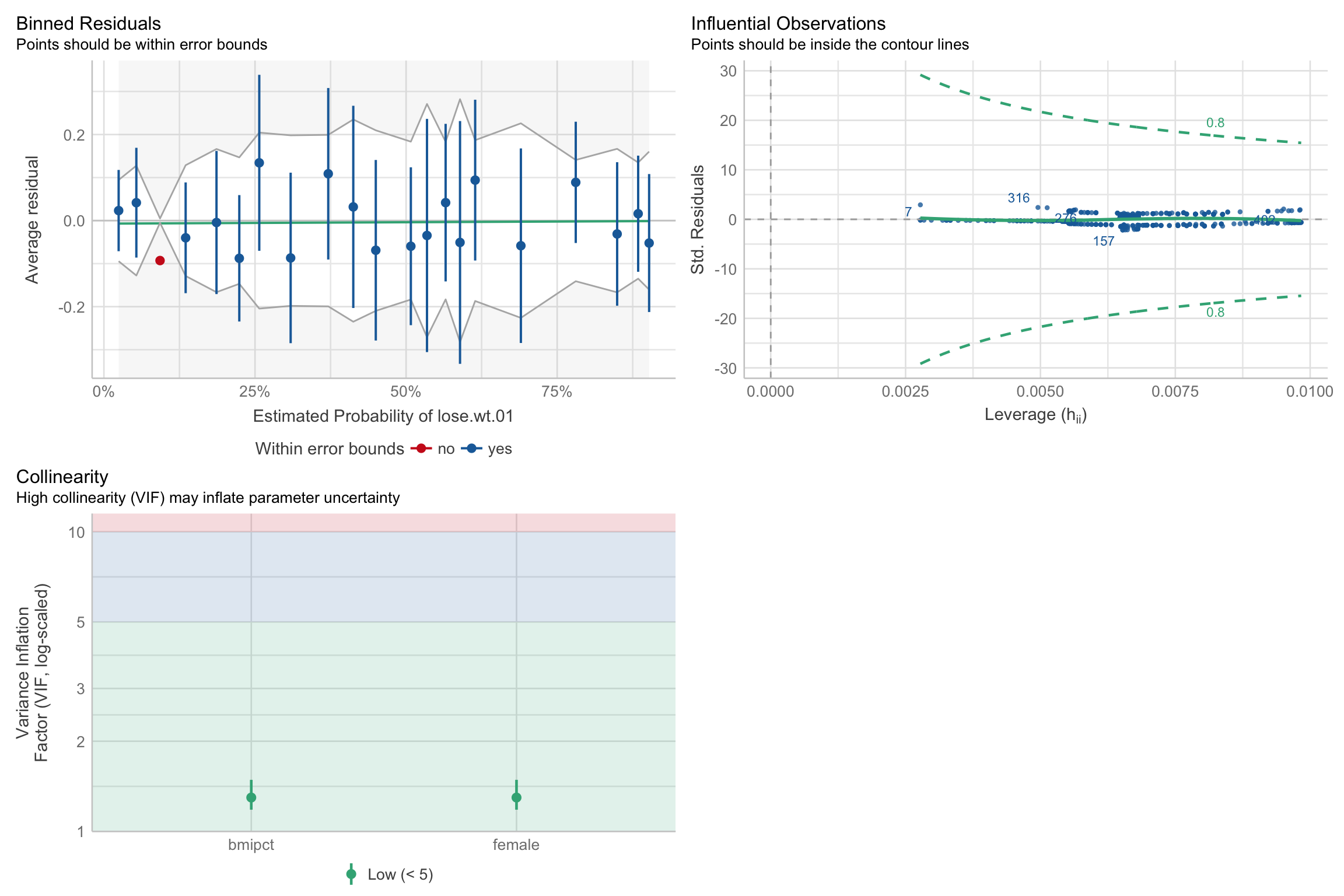
Table

fit4 %>%
  modelsummary() 

	(1)
(Intercept)	−4.259
	(0.449)
female	1.861
	(0.259)
bmipct	0.047
	(0.005)
Num.Obs.	445
AIC	469.0
BIC	481.3
Log.Lik.	−231.493
F	45.842
RMSE	0.42

Reporting

Tip

We fitted a logistic model with a logit link (estimated using ML) with sex and bmipct predicting desire to lose weight (formula: lose.wt.01 ~ 1 + female+ bmipct). The model’s explanatory power is substantial (Tjur’s \(R^2\) =0.30). The probability of females wanting to lose weight was 33% higher, b= 1.86, 95% CI [1.37, 2.38], p < .001; OR = 2.98, 95% CI [3.93, 10.9]. An increase in BMI was associated with an increased probability of wanting to lose weight, b = 0.05, 95% CI [0.04, 0.06], p < .001, OR = 1.05, 95% CI [1.04, 1.06]. Looking at the average marginal effect, 1 unit increases in BMI was associated with a 80% increase in desire to lose weight.