Beta Regression in R

Princeton University

Jason Geller, PH.D.(he/him)

2024-03-31

Today

Beta regression
- The beta distribution
  - Shapes, mean, and precision
Running a beta regression in R
- Example: reading accuracy, dyslexia, and IQ
Other beta models
- ZOIB
- Ordered beta

Package

library(betareg)
library(tidyverse)
library(marginaleffects)
library(easystats)
library(ggeffects)
library(ordbetareg)
library(knitr)

Follow along here: https://github.com/jgeller112/PSY504-Advanced-Stats-S24/blob/main/slides/09-Beta/09-Betaqmd.qmd

The beta distribution

Rates, proportions, and percentages
- Continuous distribution for 0 < y < 1
  - Important: Not including 0 or 1!
Two parameters:
- Shape 1 and Shape 2
  - Controls location, spread, skew

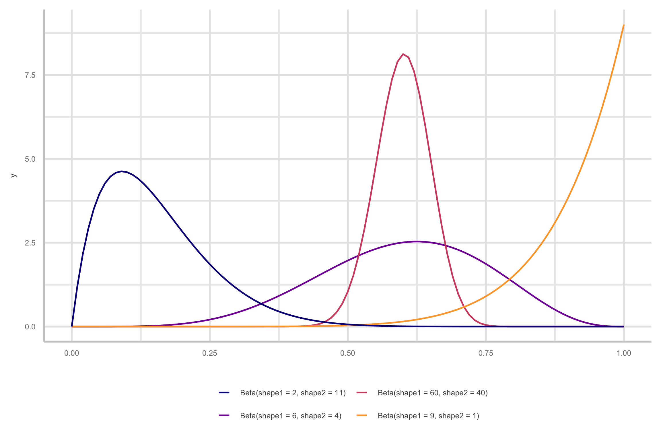
Understanding the shape parameters

Let’s say that there’s an exam worth 10 points where most people score a 6/10

\[ \frac{\text{Number correct}}{\text{Number correct} + \text{Number incorrect}} \]

\[ \frac{6}{6+4} = \frac{6}{10} \]

\[ \frac{a}{a + b} \]

Shape 1 (a)
Shape 2 (b)

Shape parameter

\(\mu\) and \(\phi\)

\(\mu\) (mean) and \(\phi\) (precision)

\[ \begin{equation} \begin{aligned}[t] \text{Shape 1:} && a &= \mu \phi \\ \text{Shape 2:} && b &= (1 - \mu) \phi \end{aligned} \qquad\qquad\qquad \begin{aligned}[t] \text{Mean:} && \mu &= \frac{a}{a + b} \\ \text{Precision:} && \phi &= a + b \end{aligned} \end{equation} \] Variance = \[ \mu \cdot (1 - \mu)/ (1 + \phi)\]

Higher \(\phi\) lower variance (narrower distribution)
Lower \(\phi\) higher variance (wider distribution)

Beta Regression

Beta regression

Here were are going to use the betareg package to run frequentist version.

Data

From Smithson & Verkuilen (2006) (taken from betareg package)
- 44 Australian primary school children
  - Dependent variable
    - accuracy : Score of test for reading accuracy
  - IVs:
    - dyslexia : (yes/no; 0.5. -0.5)
    - iq score: nonverbal IQ (z-scored)

Data

Load in data from the betareg package

Contrast code the dyslexia variable

Regular LM

model_lm <- lm(accuracy ~ dyslexia*iq,  
                      data = ReadingSkills)

model_parameters(model_lm) %>% 
  print_md()

Parameter	Coefficient	SE	95% CI	t(40)	p
(Intercept)	0.73	0.02	(0.70, 0.77)	39.36	< .001
dyslexia	-0.28	0.04	(-0.35, -0.20)	-7.38	< .001
iq	0.02	0.02	(-0.02, 0.06)	1.13	0.266
dyslexia × iq	-0.07	0.04	(-0.15, 4.13e-03)	-1.91	0.063

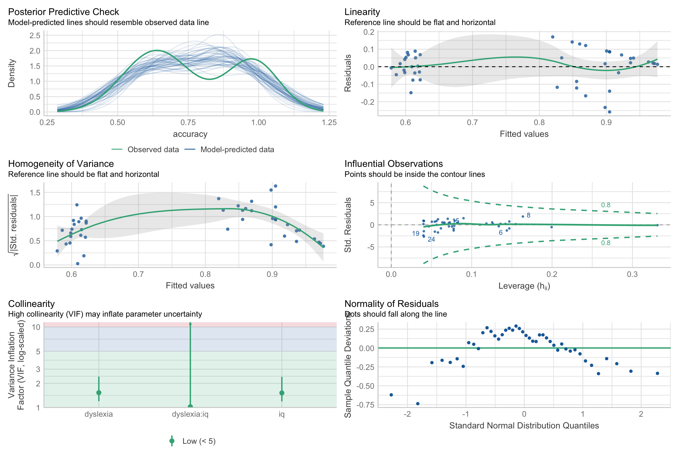
Regular LM

Models using proportions or probabilities:
- Asymmetry
- Heteoroscadacity

Beta Regression

To the rescue!

\[ accuracy_i \sim \text{Beta}(\mu_i, \phi) \]

Model has two parts
- \(\mu\)
- \(\phi\)
\[logit(\mu)= \beta_0 + \beta_1 \text{iq}_i + \beta_2 \text{dyslexia}_i + \beta_3 \text{dyslexia}_i*\text{iq}_i\]
We use the logit link so \(\mu\) is between [0,1]

Beta Regression

We model precision for each variable by inserting variables after the |

Interpretation

\(\mu\) parameters are on logit scale
- Can interpret like a logistic regression

model_parameters(model_beta, component = "conditional") %>%
  print_md()

Fixed Effects
Parameter	Coefficient	SE	95% CI	z	p
(Intercept)	1.12	0.14	(0.84, 1.40)	7.86	< .001
dyslexia	-1.48	0.29	(-2.04, -0.92)	-5.20	< .001
iq	0.49	0.13	(0.23, 0.75)	3.65	< .001
dyslexia × iq	-1.16	0.27	(-1.68, -0.64)	-4.38	< .001

Interpretation

\(\phi\) (precision) parameter is on log scale so we can exp to get back to original metric

model_parameters(model_beta, exponentiate = TRUE,  component = "precision") %>%
  print_md()

Fixed Effects
Parameter	Coefficient	SE	95% CI	z	p
(Intercept)	27.23	6.07	(17.60, 42.14)	14.84	< .001
dyslexia	32.89	17.25	(11.76, 91.96)	6.66	< .001
iq	3.42	0.91	(2.02, 5.77)	4.60	< .001

Marginal effects

Because means are on logit scale we can do what we did with logistic regression and evaluate probabilities

#probs 
avg_predictions(model_beta, variables="dyslexia") %>%
  kable()

dyslexia	estimate	std.error	statistic	p.value	s.value	conf.low	conf.high
-0.5	0.8230004	0.0492736	16.70268	0	205.6341	0.7264260	0.9195748
0.5	0.5940562	0.0105573	56.26962	0	Inf	0.5733642	0.6147481

Marginal effects

#get differnece 
avg_comparisons(model_beta) %>%
  kable()

term	contrast	estimate	std.error	statistic	p.value	s.value	conf.low	conf.high
dyslexia	+1	-0.2450026	0.0524356	-4.672451	0.0000030	18.358064	-0.3477744	-0.1422308
iq	+1	0.0274402	0.0130397	2.104362	0.0353469	4.822273	0.0018829	0.0529975

Note

For 1-unit increase in iq there is an increase of 2 percentage points on reading accuracy
Dyslexia decreases reading accuracy by 25 percentage points

Model comparison

LRT

## use type 3 if interactions important
car::Anova(model_beta, type="III") %>% 
  kable()

	Df	Chisq	Pr(>Chisq)
(Intercept)	1	61.84003	0.0000000
dyslexia	1	26.99045	0.0000002
iq	1	13.34291	0.0002594
dyslexia:iq	1	19.18920	0.0000118

Interaction

Simple slopes analysis comparing AME for iq at each level of dyslexia variable

marginaleffects::avg_slopes(
    model_beta,
    variables  = "iq", 
    by="dyslexia") %>%
  kable()

term	contrast	dyslexia	estimate	std.error	statistic	p.value	s.value	conf.low	conf.high	predicted_lo	predicted_hi	predicted
iq	mean(dY/dX)	-0.5	0.0955828	0.0347942	2.747086	0.0060127	7.377765	0.0273873	0.1637782	0.9397779	0.9397997	0.9397888
iq	mean(dY/dX)	0.5	-0.0225628	0.0115910	-1.946572	0.0515861	4.276873	-0.0452808	0.0001552	0.5961558	0.5961475	0.5961517

Note

For those with dyslexia, an increase in iq deceases reading accuracy by 2 percentage points, \(b\) = -.02, SE = 0.01, 95% CI [-0.04, .00], p = .051. However, this is not statistically significant. For those without dyslexia, reading accuracy improves by 10 percentage points for 1 unit increase in iq, \(b\) = -.02, SE = 0.01, 95% CI [0.027, .163] p = .006.

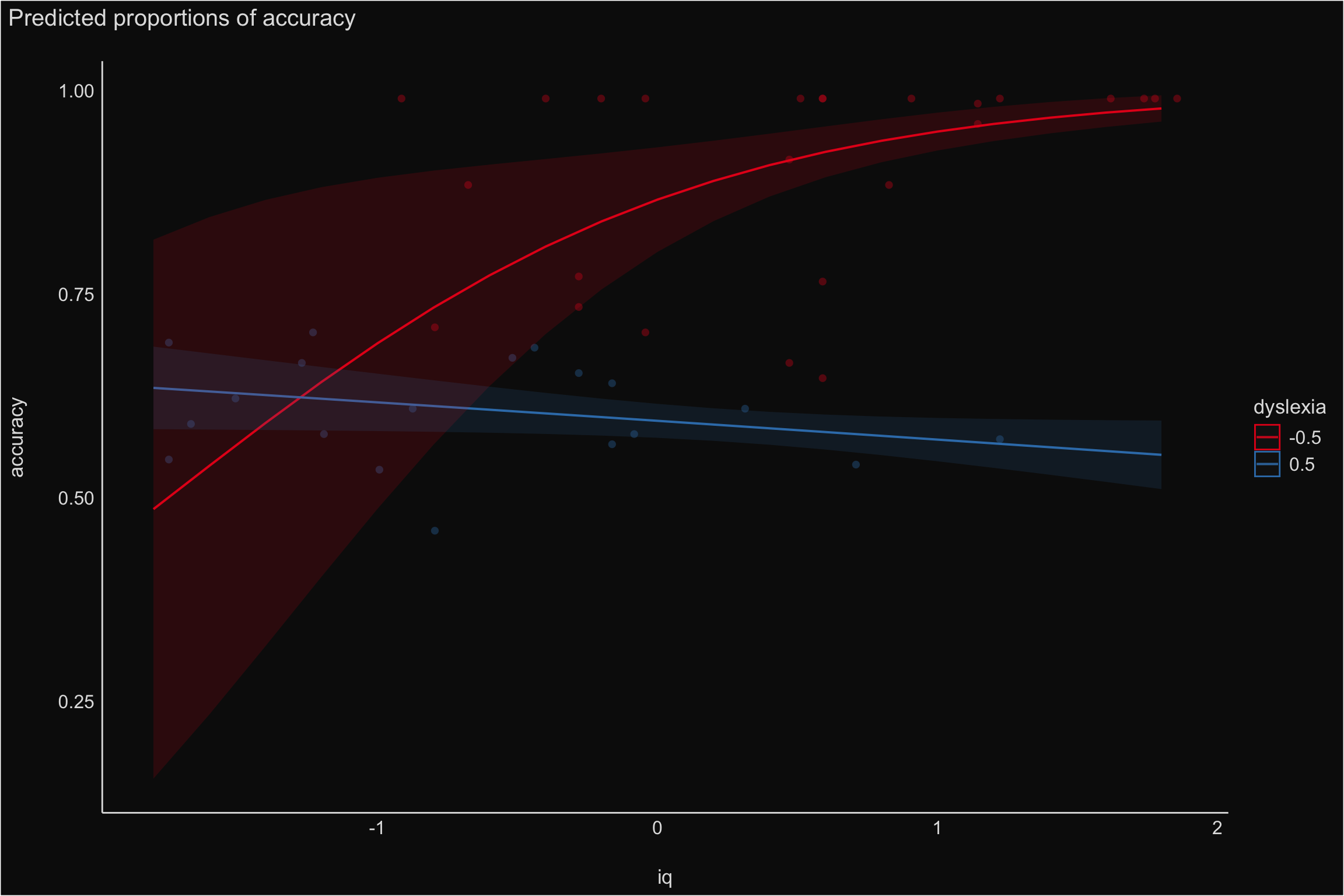
Visualization - Interaction

ggemmeans(model_beta, terms=c("iq", "dyslexia")) %>% 
  plot(show_data=TRUE)+ theme_blackboard()

IQ and Accuracy does not seem to be related to dyslexia

Model Comparisons

Do we need a precision parameters for each variable?

# before | is mean after is phi/variance
model_beta <- betareg(accuracy ~ dyslexia*iq  |dyslexia + iq , 
                      data = ReadingSkills, 
                      link = "logit")

# estimate only one phi
# before | is mean after is phi/variance
model_beta_nophi <- betareg(accuracy ~ dyslexia*iq , 
                      data = ReadingSkills, 
                      link = "logit")

test_likelihoodratio(model_beta, model_beta_nophi)

# Likelihood-Ratio-Test (LRT) for Model Comparison (ML-estimator)

Name             |   Model | df | df_diff |  Chi2 |      p
----------------------------------------------------------
model_beta       | betareg |  7 |         |       |       
model_beta_nophi | betareg |  5 |      -2 | 29.10 | < .001

\(\phi\) for each variable is warranted

Other beta models

More complex models like zero-one inflated betas and ordered betas cannot be fit in frequentist framework

ZOIB

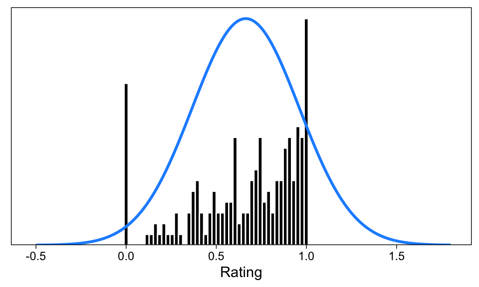
if you have zeros and one in your data

ZOIB

Three processes

A logistic regression model that predicts if outcome is either (1) 0 or 1 or (2) not exactly 0 or 1 (\(\alpha\) or zoi in brms)
A logistic regression model that predicts if the 0 or 1 outcomes are either (1) 0 or (2) 1 (\(\gamma\) or coi in brms)
A beta regression model that predicts the non-extreme (0 or 1) values) (\(\mu\) and \(\phi\))

brm(
  bf(
    outcome ~ covariates,  # The mean of the 0-1 values, or mu
    phi ~ covariates,  # The precision of the 0-1 values, or phi
    zoi ~ covariates,  # The zero-or-one-inflated part, or alpha
    coi ~ covariates  # The one-inflated part, conditional on the 0s, or gamma
  ),
  data = whatever,
  family = zero_one_inflated_beta(),
  ...
)

ZOIB - Output

##  Family: zero_one_inflated_beta 
##   Links: mu = logit; phi = log; zoi = logit; coi = logit 
## Formula: Rating ~ group 
##          phi ~ group
##          zoi ~ group
##          coi ~ group
##    Data: dat (Number of observations: 100) 
##   Draws: 4 chains, each with iter = 2000; warmup = 1000; thin = 1;
##          total post-warmup draws = 4000
## 
## Population-Level Effects: 
##               Estimate Est.Error l-95% CI u-95% CI Rhat Bulk_ESS Tail_ESS
## Intercept         0.33      0.16     0.03     0.64 1.00     7221     2600
## phi_Intercept     1.50      0.24     1.00     1.94 1.00     6306     3106
## zoi_Intercept    -0.80      0.32    -1.44    -0.18 1.00     7341     2983
## coi_Intercept     0.62      0.56    -0.40     1.75 1.00     6324     3166
## groupB            0.91      0.21     0.50     1.32 1.00     6770     2984
## phi_groupB        0.48      0.33    -0.15     1.14 1.00     5750     2654
## zoi_groupB        0.08      0.43    -0.75     0.91 1.00     7812     3178
## coi_groupB       -0.87      0.75    -2.35     0.52 1.00     6093     2866
## 
## Draws were sampled using sampling(NUTS). For each parameter, Bulk_ESS
## and Tail_ESS are effective sample size measures, and Rhat is the potential
## scale reduction factor on split chains (at convergence, Rhat = 1).

Ordered beta

ZOIB can become complex with lots of parameters to estimate!
- Can take a long time to run
Ordered beta regression is a special case of ZOIB
- Robert Kubinec developed it
- It combines ordinal and beta regression

library(ordbetareg)

Ordered beta regression

We can create three ordered categories to use as an outcome variable: (1) exactly 0 (cutzero), (2) somewhere between 0 and 1, and (3) exactly 1 (cutone)
- 1 and 3 are modeled as with ordinal logits (exactly 0 and exactly 1) and 2 is modeled as a beta logits
- We can just interpret this similarly to beta regression while still including zeros and ones

Ordered beta

m_full_ordbeta <- ordbetareg(
  bf(
    province_count ~ 
      issue_arts_and_culture), 
  data = data,
  true_bounds = c(1, 32), # does not have to be between 0-1/0-100
  ...
)

##  Family: ord_beta_reg 
##   Links: mu = identity; phi = identity; cutzero = identity; cutone = identity 
## Formula: province_count ~ issue_arts_and_culture + issue_education + issue_industry_association + issue_economy_and_trade + issue_charity_and_humanitarian + issue_general + issue_health + issue_environment + issue_science_and_technology + local_connect + years_since_law + year_registered_cat 
##    Data: data (Number of observations: 593) 
##   Draws: 4 chains, each with iter = 2000; warmup = 1000; thin = 1;
##          total post-warmup draws = 4000
## 
## Population-Level Effects: 
##                                    Estimate Est.Error l-95% CI u-95% CI Rhat Bulk_ESS Tail_ESS
## Intercept                             -0.23      0.33    -0.89     0.44 1.00     1039     1305
## issue_arts_and_cultureTRUE             1.31      0.43     0.47     2.16 1.00     1790     2390
## Family Specific Parameters: 
##         Estimate Est.Error l-95% CI u-95% CI Rhat Bulk_ESS Tail_ESS
## phi         2.19      0.20     1.82     2.62 1.00     3657     2577
## cutzero    -1.26      0.13    -1.53    -1.00 1.00     2438     2762
## cutone      0.34      0.07     0.19     0.47 1.00     3377     2878
## 
## Draws were sampled using sample(hmc). For each parameter, Bulk_ESS
## and Tail_ESS are effective sample size measures, and Rhat is the potential
## scale reduction factor on split chains (at convergence, Rhat = 1).

Summary

Beta regression is an excellent choice for modeling percentages, proportions, and ratios
If you have 0s and 1s, alternatives exist
- ZOIB or ordered beta regression (Bayesian framework)
Not a whole lot of examples using these kind of models, but hopefully this gives you a good start!

Beta Regression in R

Today

Package

The beta distribution

Understanding the shape parameters

Shape parameter

\(\mu\) and \(\phi\)

Beta Regression

Beta regression

Data

Data

Regular LM

Regular LM

Regular LM

Beta Regression

Beta Regression

Interpretation

Interpretation

Marginal effects

Marginal effects

Model comparison

LRT

Interaction

Visualization - Interaction

Model Comparisons

Other beta models

ZOIB

ZOIB

ZOIB - Output

Ordered beta

Ordered beta regression

Ordered beta

Summary

Fin