Mediation Analysis in R

Princeton University

Jason Geller, PH.D.(he/him)

2024-04-09

Today

Testing mediation in R
- Classical approach to testing mediation (Baron and Kenny)
- Joint significance
- Sobel
- Bootstrapped approach to testing mediation (preferred approach)
Other models:
- Multiple mediators
- Within-subject mediation
Reporting mediation results

Eclipse

Packages

#devtools::install_github("dustinfife/flexplot")
library(tidyverse)
library(lavaanPlot)
library(easystats)
library(lavaan)
library(kableExtra)
library(broom)
library(flextable)
library(flexplot)
library(mediation)
library(JSmediation)
library(processR)
library(MeMoBootR)
library(broom)

options(scipen = 999) # get rid sci notation

Follow along here: https://github.com/jgeller112/PSY504-Advanced-Stats-S24/blob/main/slides/10-mediation/mediation.qmd

Is mediation f***ed?

Mediation is a hard causal inference task!
- Manipulation of and random assignment of X affords causal inference/causal claims
  - However, we rarely do the same for M
    - Mediation analysis requires theory and subsequent experiments to test mediator

Is mediation f***ed?

Julia Rohrer’s talk delves into some of these issues

Introduction to DAG analysis
- Slides: https://osf.io/9d4ef
- Video:https://drive.google.com/file/d/1evOsN_LLl013yc015REAMRyQWfuSoeRb/view?usp=drivesdk

Note

Bullock, J. G., Green, D. P., & Ha, S. E. (2010). Yes, but what’s the mechanism? (don’t expect an easy answer). Journal of personality and social psychology, 98(4), 550–558. https://doi.org/10.1037/a0018933

Mediation: Example

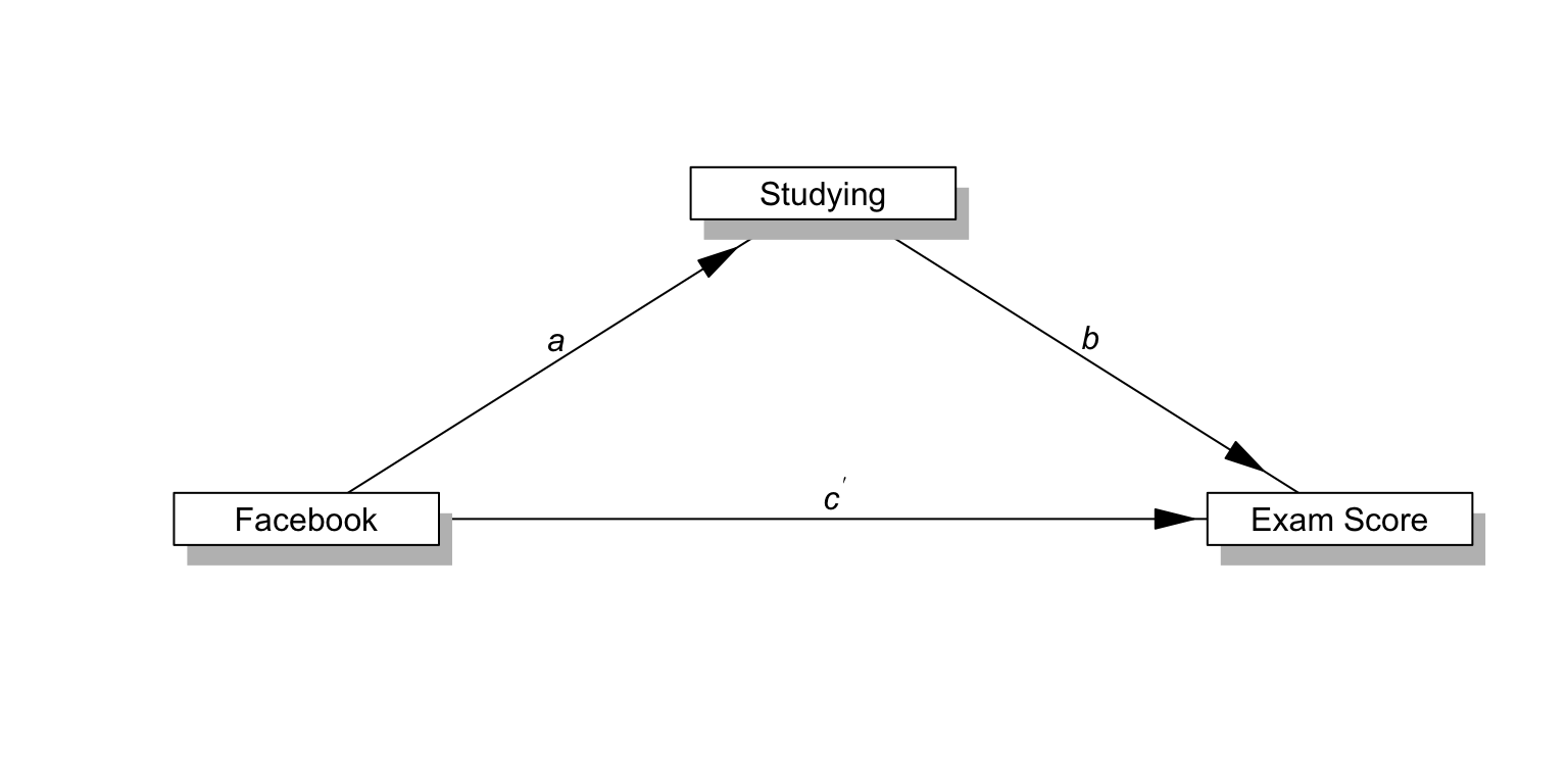
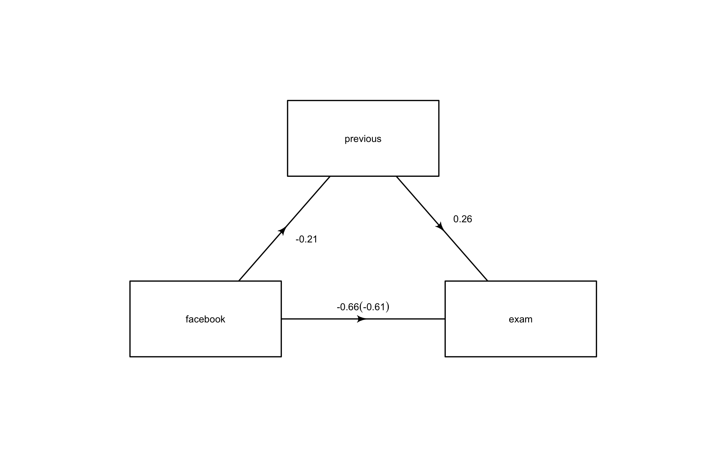
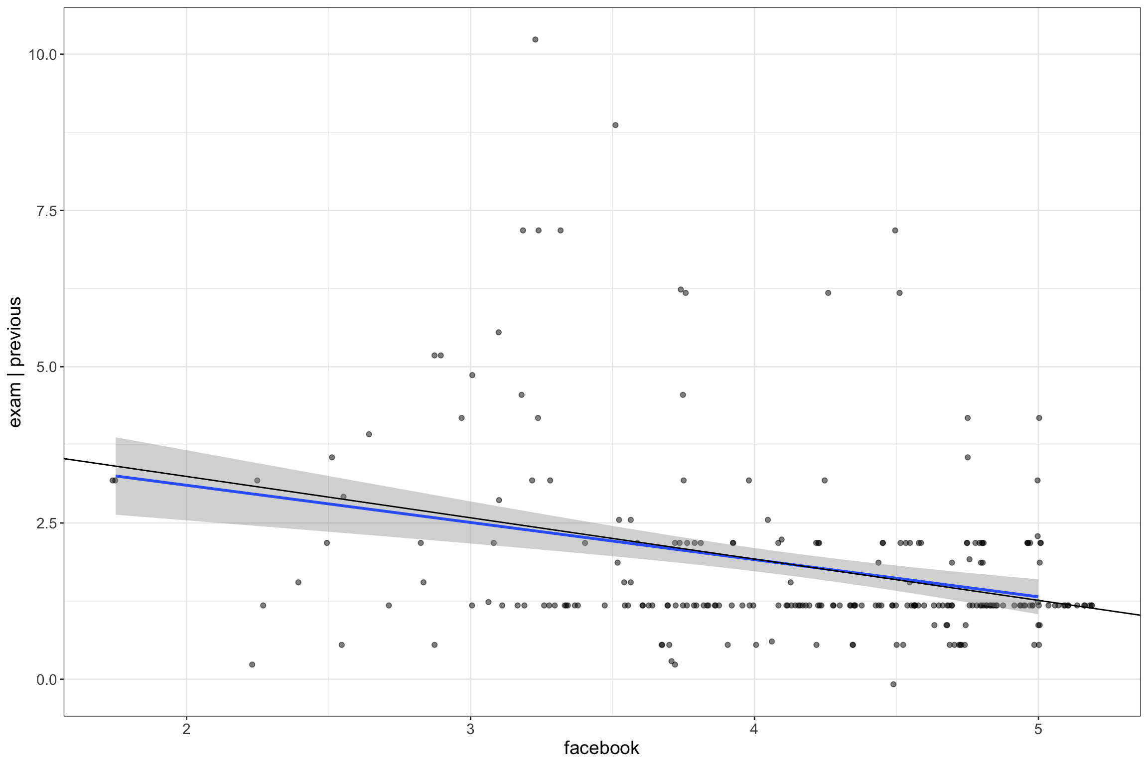
Does study time mediate the relationship between Facebook usage and exam scores?
- Implying that the overuse of Facebook prevents people from studying, so they do differently on their exam

Load packages

library(MeMoBootR) # mediation analysis #download from gihub
library(JSmediation) # mediation analysis
library(flexplot) # mediate_plot function
library(lavaan) # SEM and mediation 
#library(tidySEM)# plot models from lavaan
library(processR) # path model figs`

Load data

previous	facebook	exam
3	3.666667	1
2	5.000000	1
1	4.000000	2
1	4.500000	7
1	4.500000	6
1	4.500000	1

Testing Mediation

Causal Steps - Baron & Kenny (1986)

Mediation is tested through three regression models:

Regression 1
Regression 2
Regression 3

Predicting the outcome from the predictor variable
X -> Y
c path : total effect

Predicting the mediator from the predictor variable
X -> M
a path

Predicting the outcome from both the predictor variable and the mediator
X+M→Y
b path
c’ (c-prime) path: direct effect

Mediation Paths

Paths
c: “total effect” of X on Y	Total effect = direct effect + indirect effect
a x b = “indirect effect” of X on Y (our mediation effect)	indirect effect = total effect - direct effect
\(c^\prime\) = “direct effect” of X on Y

Why take the product of the two coefficients?

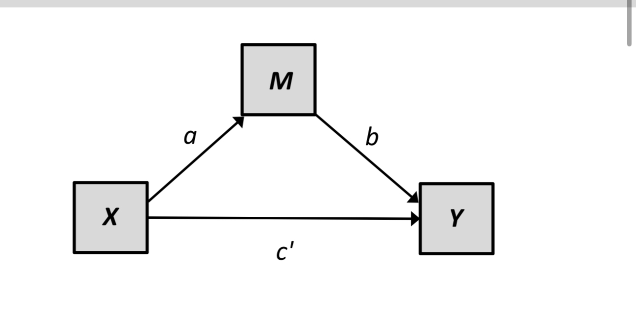
An intuitive explanation:
- A 1 unit increase in M corresponds to a b unit increase in Y holding X constant
  - How much does X change M?
    - a
So if a = 1/2, X changes M by 1/2, which then changes Y by b, the indirect effect is (1/2) × b

Causal Steps - Baron & Kenny (1986)

Traditionally, to show mediation ALL these conditions must be met:
- X must significantly predict Y in Step 1
- X must significantly predict M in Step 2
- M must significantly predict Y controlling for X in Step 3
- The effect of X on Y must be reduced in Step 3
  - If X is no longer significant, you have “full mediation”
  - If X is still significant, then you have “partial mediation”
    - Not really used in anymore

Mediation: c path

Parameter	Coefficient	SE	CI	CI_low	CI_high	t	df_error	p
(Intercept)	4.5679439	0.5389142	0.95	3.5062701	5.6296178	8.476199	237	0.0000000
facebook	-0.6611852	0.1280633	0.95	-0.9134729	-0.4088974	-5.162956	237	0.0000005

The c path (total effect): X –> Y:

\(b = -0.66, t(237) = -5.16, 95\% CI[-0.91, -0.41], p < .001\)

Mediation: a path

Parameter	Coefficient	SE	CI	CI_low	CI_high	t	df_error	p
(Intercept)	2.4466495	0.4095586	0.95	1.6398092	3.2534899	5.973869	237	0.0000000
facebook	-0.2108046	0.0973243	0.95	-0.4025358	-0.0190734	-2.166002	237	0.0313087

The a path: X –> M:

\(b = -0.21, t(237) = -2.16, 95\% CI[-0.40, -0.02], p = .031\)

Mediation: b, c’ path

Add in the b (M –> Y) and c’ (direct) paths: X + M –> Y

Parameter	Coefficient	SE	CI	CI_low	CI_high	t	df_error	p
(Intercept)	3.9329387	0.5679094	0.95	2.8141192	5.0517583	6.925292	236	0.0000000
facebook	-0.6064728	0.1270523	0.95	-0.8567744	-0.3561712	-4.773409	236	0.0000032
previous	0.2595407	0.0839713	0.95	0.0941117	0.4249697	3.090828	236	0.0022357

c’ Path: \(b = -0.61, t(237) = -4.77, 95\% CI[-0.86, -0.36], p < .001\)
b Path: \(b = 0.26, t(237) = 3.09, 95\% CI[0.09, 0.42], p = .002\)

Mediation: interpretation

Facebook usage negatively impacts exam scores (c path = -.66)
Facebook usage negatively impacts previous study time (a path = -.21)
Controlling for Facebook time, previous study time positively impacts exam scores (b path = .26)
Controlling for previous study time, Facebook usage negatively impacts exam scores (c’ path = -0.61)

Do we have mediation here?

Causal Steps - Baron & Kenny (1986)

Traditionally, to show mediation ALL these conditions must be met:
- X must significantly predict Y in Step 1 ✅
- X must significantly predict M in Step 2 ✅
- M must significantly predict Y controlling for X in Step 3 ✅
- The effect of X on Y must be reduced in Step 3
  - If X is no longer significant, you have “full mediation”
  - If X is still significant, then you have “partial mediation” ✅
    - Not really used in anymore

Issues with causal steps

Indirect effect is inferred rather than directly estimated

Failure to meet a criterion results in game over!

If total effect (path c) is not statistically significant, game does not begin

Joint significance test

An edited version of causal steps approach
- If a path and b path are significant
  - Mediation!
Some issues:
- Indirect effect is inferred rather than directly estimated
- Failure to meet a criterion results in game over!

Note

Yzerbyt, V., Muller, D., Batailler, C., & Judd, C. M. (2018). New recommendations for testing indirect effects in mediational models: The need to report and test component paths. Journal of Personality and Social Psychology, 115(6), 929–943. doi: 10.1037/pspa0000132

Testing mediation: Sobel test

So, did mediation happen? Is a change from 0.66 to 0.61 important?
The Sobel Test:

\[Z = \frac{a \times b}{\sqrt{b^2 \times SE_a^2 + a^2 \times SE_b^2}}\]
- If the indirect effect is larger than the error, we would conclude that the addition of the M variable changed the c path

Sobel Test

Sobel test

library(bda)
#conducts sobel test
mediation.test(master$previous,master$facebook,master$exam)

              Sobel      Aroian     Goodman
z.value -1.77380460 -1.71464047 -1.83954863
p.value  0.07609548  0.08641116  0.06583453

Z = -1.77, p = .08
- We would conclude that no mediation had occurred

Note

Other tests listed use slightly different denominator formula

Sobel test

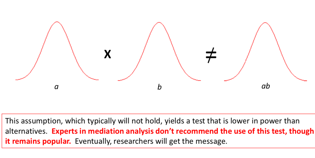
Serious problem!
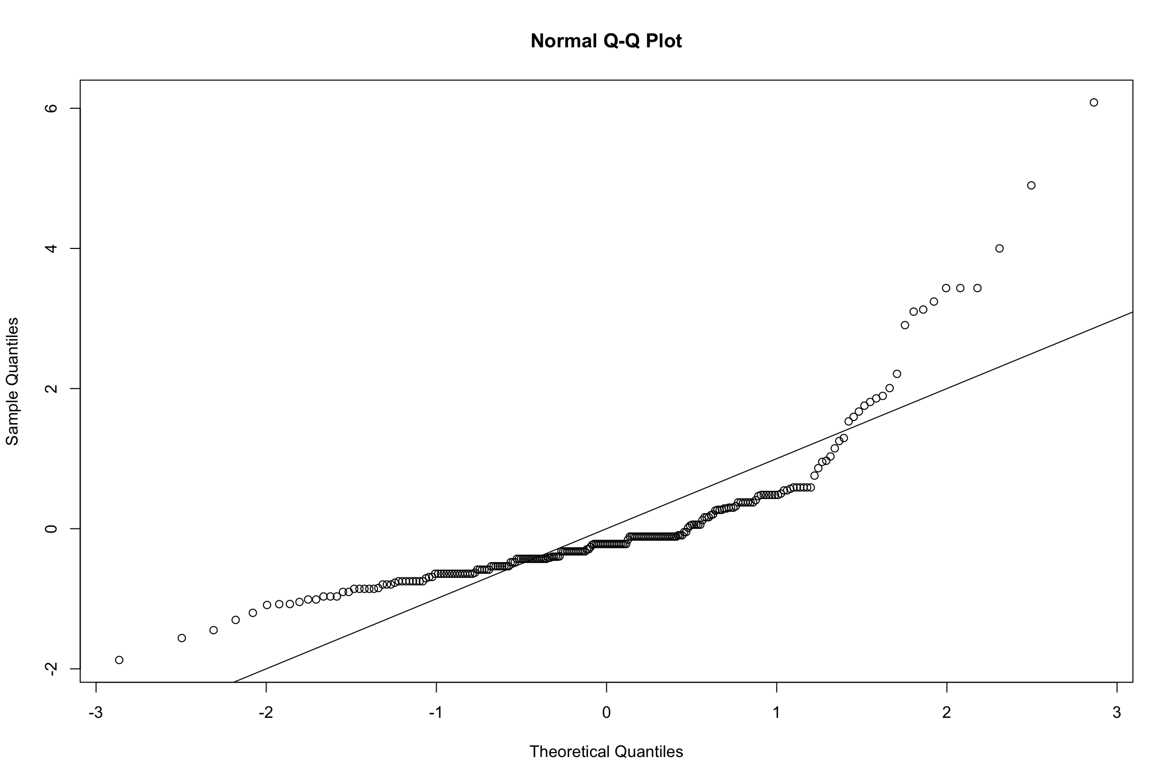
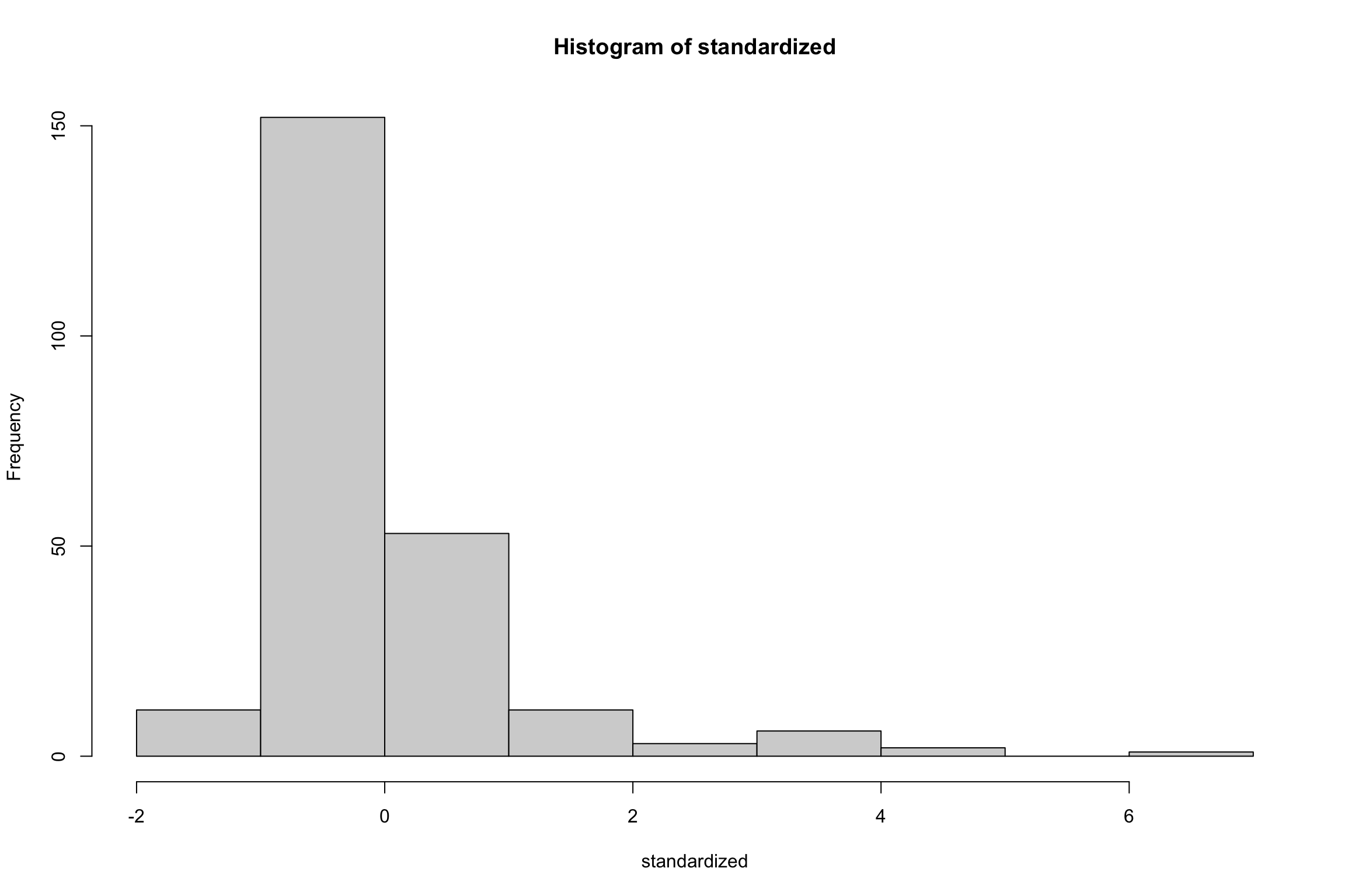
- Assumes indirect effect is normally distributed
  - Not always the case

Mediation: Bootstrapping

Testing significance of indirect effect (a x b)
- Does not assume distribution is normal
- More sensitive test = Higher power!

Mediation: Bootstrapping

What it is:
- A computer based method for deriving the probability distribution for any random variable
When to use it:
- You do not know the distribution of your variable(s)
How to do it:
- Run your analysis a bunch of times with a slightly different set of observations each time

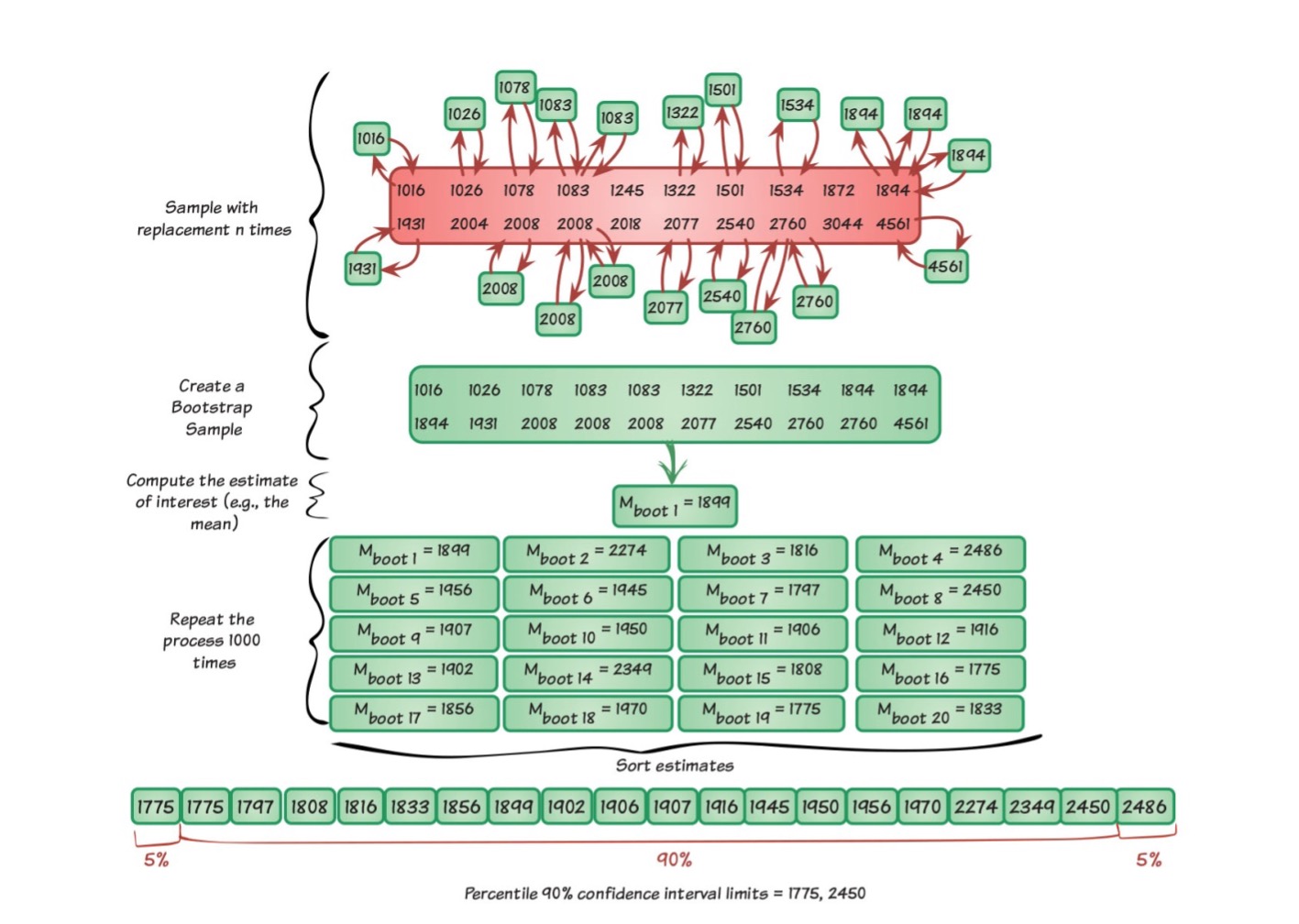
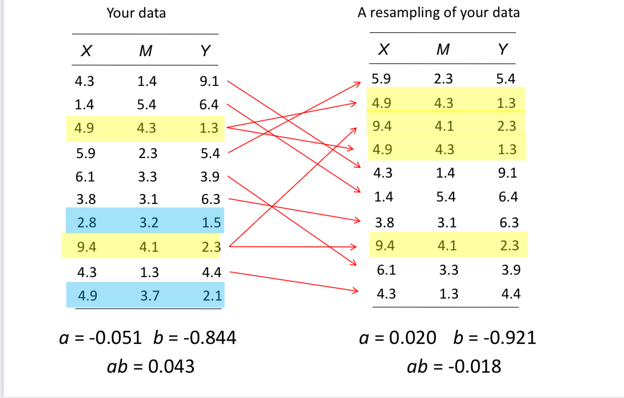
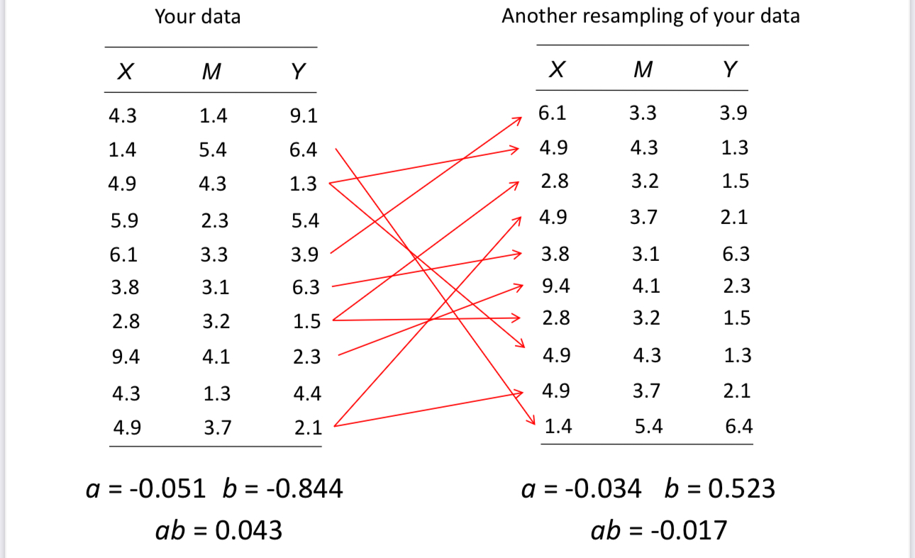
Bootstrap: Overview

Take a random sample of size n from the sample with replacement
Estimate the indirect effect in this “resample”
Repeat (1) and (2) a total of k times, where k is at least 1,000. The larger k, the better. I recommend at least 10,000
Use distribution of the indirect effect over multiple resamples as an approximation of the sampling distribution of the indirect effect

Bootstrap: Overview

The Bootstrapped CI

Using the bootstrap sample we can calculate 95% CI
- Percentile bootstrap
  - Find the 2.5th and 97.5th percentiles of the distribution of the statistic
If 0 is included, no mediation

Note

Variations exist (e.g., ‘bias corrected’ or ‘bias-corrected and accelerated’ confidence intervals but they do not perform as well as percentile.)

Mediation: All together + bootstrapping

Do it all with one function
- The MeMoBootR package (developed by Erin Buchanon) gives you data screening, each step of the mediation, and the bootstrapping results!
  - The data screening does not include accuracy or missing data, so that should be completed first

devtools::install_github("doomlab/MeMoBootR")
#library(MeMoBootR)
#no missing data allowed
med_results <- mediation1(y = "exam",
                          x = "facebook", 
                          m = "previous", nboot = 1000, 
                          df = master)

med_results$datascreening$linearity

med_results$datascreening$normality

med_results$datascreening$homogen

Mediation: MeMoBootR

For each of our stages of mediation, you can print out the models:

Step 1
Step 2
Step 3

model_parameters(med_results$model1) %>% kable()

Parameter	Coefficient	SE	CI	CI_low	CI_high	t	df_error	p
(Intercept)	4.5679439	0.5389142	0.95	3.5062701	5.6296178	8.476199	237	0.0000000
facebook	-0.6611852	0.1280633	0.95	-0.9134729	-0.4088974	-5.162956	237	0.0000005

model_parameters((med_results$model2)) %>% kable()

Parameter	Coefficient	SE	CI	CI_low	CI_high	t	df_error	p
(Intercept)	2.4466495	0.4095586	0.95	1.6398092	3.2534899	5.973869	237	0.0000000
facebook	-0.2108046	0.0973243	0.95	-0.4025358	-0.0190734	-2.166002	237	0.0313087

model_parameters(med_results$model3) %>% kable()

Parameter	Coefficient	SE	CI	CI_low	CI_high	t	df_error	p
(Intercept)	3.9329387	0.5679094	0.95	2.8141192	5.0517583	6.925292	236	0.0000000
facebook	-0.6064728	0.1270523	0.95	-0.8567744	-0.3561712	-4.773409	236	0.0000032
previous	0.2595407	0.0839713	0.95	0.0941117	0.4249697	3.090828	236	0.0022357

Mediation: MeMoBootR

Next, you can get the Sobel test results:

med_results$indirect.effect

   facebook 
-0.05471237

med_results$z.score

facebook 
-1.71464

med_results$p.value

  facebook 
0.08641116

Bootstrapping

Last, let’s get the bootstrapped results:

med_results$boot.results


ORDINARY NONPARAMETRIC BOOTSTRAP


Call:
boot(data = finaldata, statistic = indirectmed, R = nboot, formula2 = allformulas$eq2, 
    formula3 = allformulas$eq3, x = x, med.var = m)


Bootstrap Statistics :
       original       bias    std. error
t1* -0.05471237 -0.001450445  0.03794187

Bootstrapping

Returns several type of cis
- Percentile bootstrap

med_results$boot.ci$percent %>% kable()

conf
0.95	25.03	975.98	-0.1459171	-0.000731

The indirect effect would be reported as: b = -0.05, 95% CI[-0.147, -0.001]

Mediation visualization

med_results$diagram

Note

No good programs to create nice looking path models

Mediation visualization

library(flexplot) # mediation plot

mediate_plot(exam~previous +facebook,data=master)

JSmediation

Incorporates easystats

library(JSmediation)

mediation_fit <- mdt_simple(master,
             IV =facebook,
             DV = exam,
             M  = previous)

JSmediation results

# Mediation Results
mediation_fit

Test of mediation (simple mediation)
==============================================

Variables:

- IV: facebook 
- DV: exam 
- M: previous 

Paths:

====  ==============  =====  =======================
Path  Point estimate     SE  APA                    
====  ==============  =====  =======================
a             -0.211  0.097  t(237) = 2.17, p = .031
b              0.260  0.084  t(236) = 3.09, p = .002
c             -0.661  0.128  t(237) = 5.16, p < .001
c'            -0.606  0.127  t(236) = 4.77, p < .001
====  ==============  =====  =======================

Indirect effect index:

Indirect effect index is not computed by default.
Please use add_index() to compute it.

Fitted models:

- X -> Y 
- X -> M 
- X + M -> Y

JSmediation: Indirect effect

# Testing Indirect Effect with `JSmediation`
model_fit_with_index <- add_index(mediation_fit)
model_fit_with_index

Test of mediation (simple mediation)
==============================================

Variables:

- IV: facebook 
- DV: exam 
- M: previous 

Paths:

====  ==============  =====  =======================
Path  Point estimate     SE  APA                    
====  ==============  =====  =======================
a             -0.211  0.097  t(237) = 2.17, p = .031
b              0.260  0.084  t(236) = 3.09, p = .002
c             -0.661  0.128  t(237) = 5.16, p < .001
c'            -0.606  0.127  t(236) = 4.77, p < .001
====  ==============  =====  =======================

Indirect effect index:

- type: Indirect effect 
- point estimate: -0.0547 
- confidence interval:
  - method: Monte Carlo (5000 iterations)
  - level: 0.05 
  - CI: [-0.129; -0.00377]

Fitted models:

- X -> Y 
- X -> M 
- X + M -> Y

Note

Take note of defaults and how how CIs are estimated. Here they use Monte Carlo CIs

JSmediation results: Assumptions

Step 1
Step 2
Step 3

first_model <- extract_model(mediation_fit, step = 1)
performance::check_model(first_model)

second_model <- extract_model(mediation_fit, step = 2)
performance::check_model(second_model)

third_model <- extract_model(mediation_fit, step = 3)
performance::check_model(third_model)

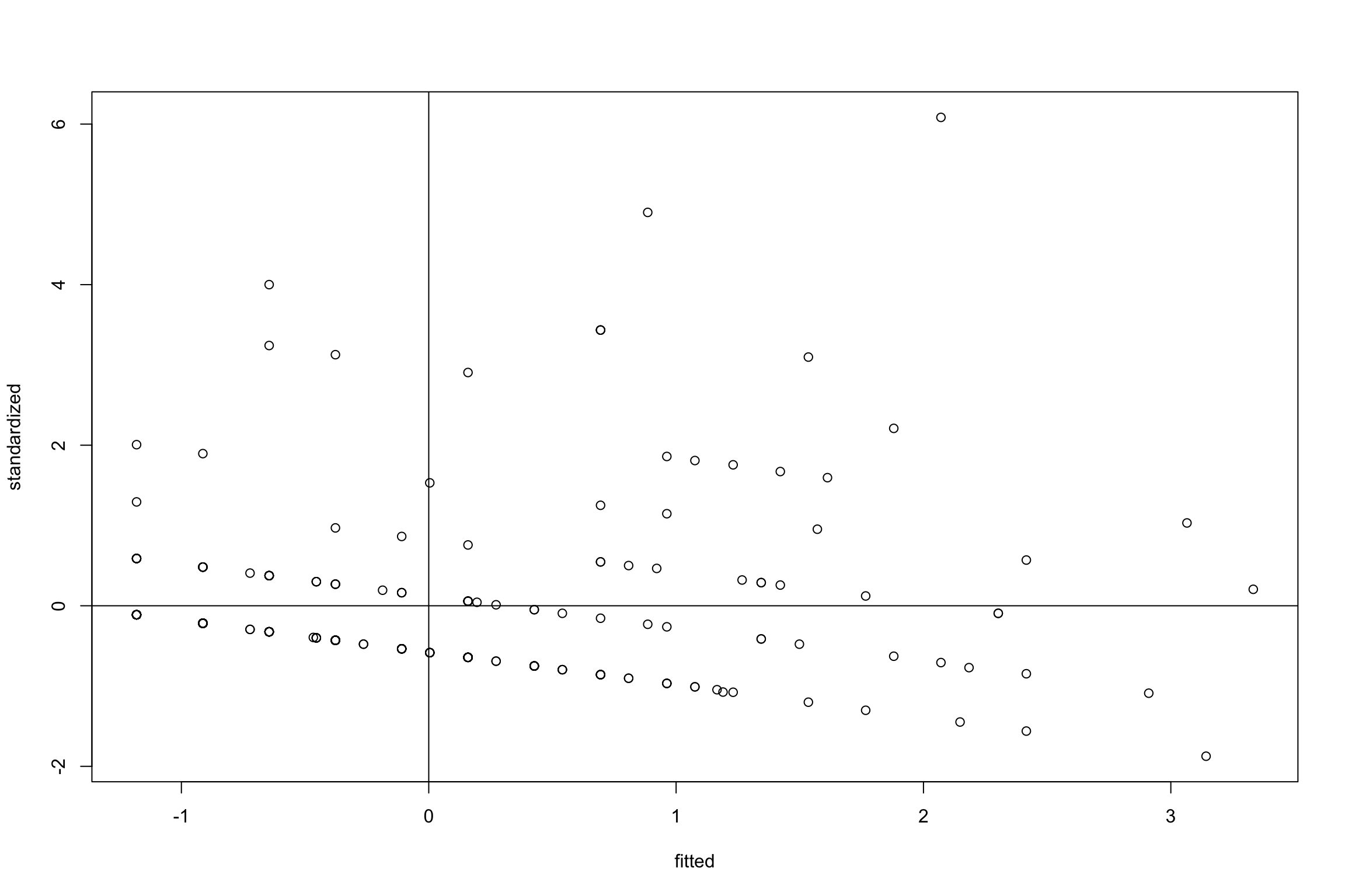
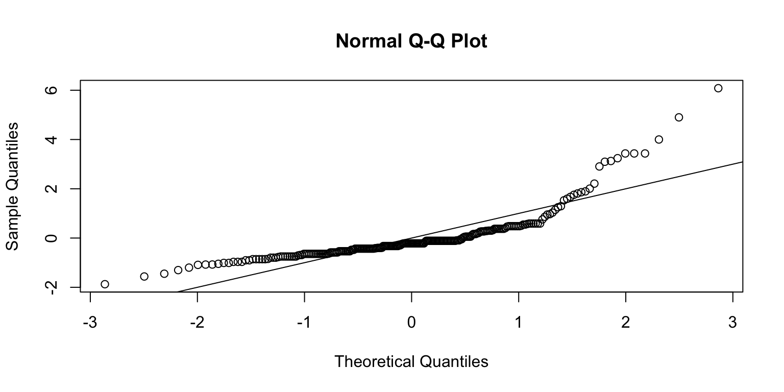
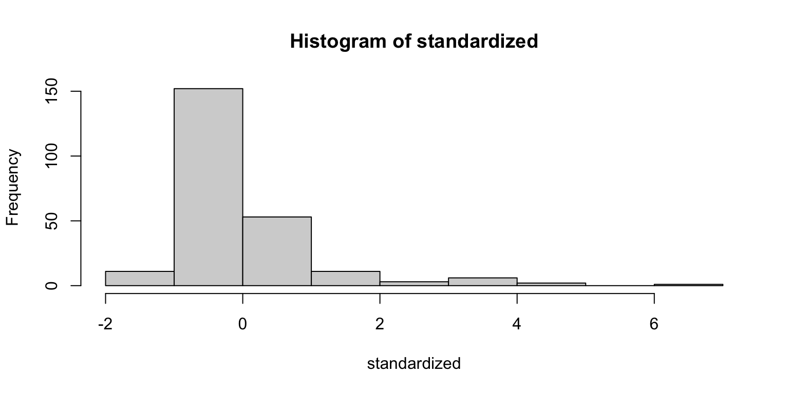
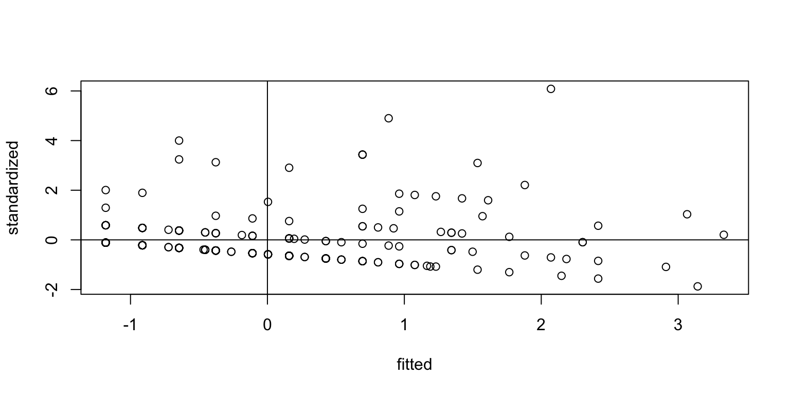
JSmediation results: Assumptions

JSmediation::check_assumptions(model_fit_with_index)

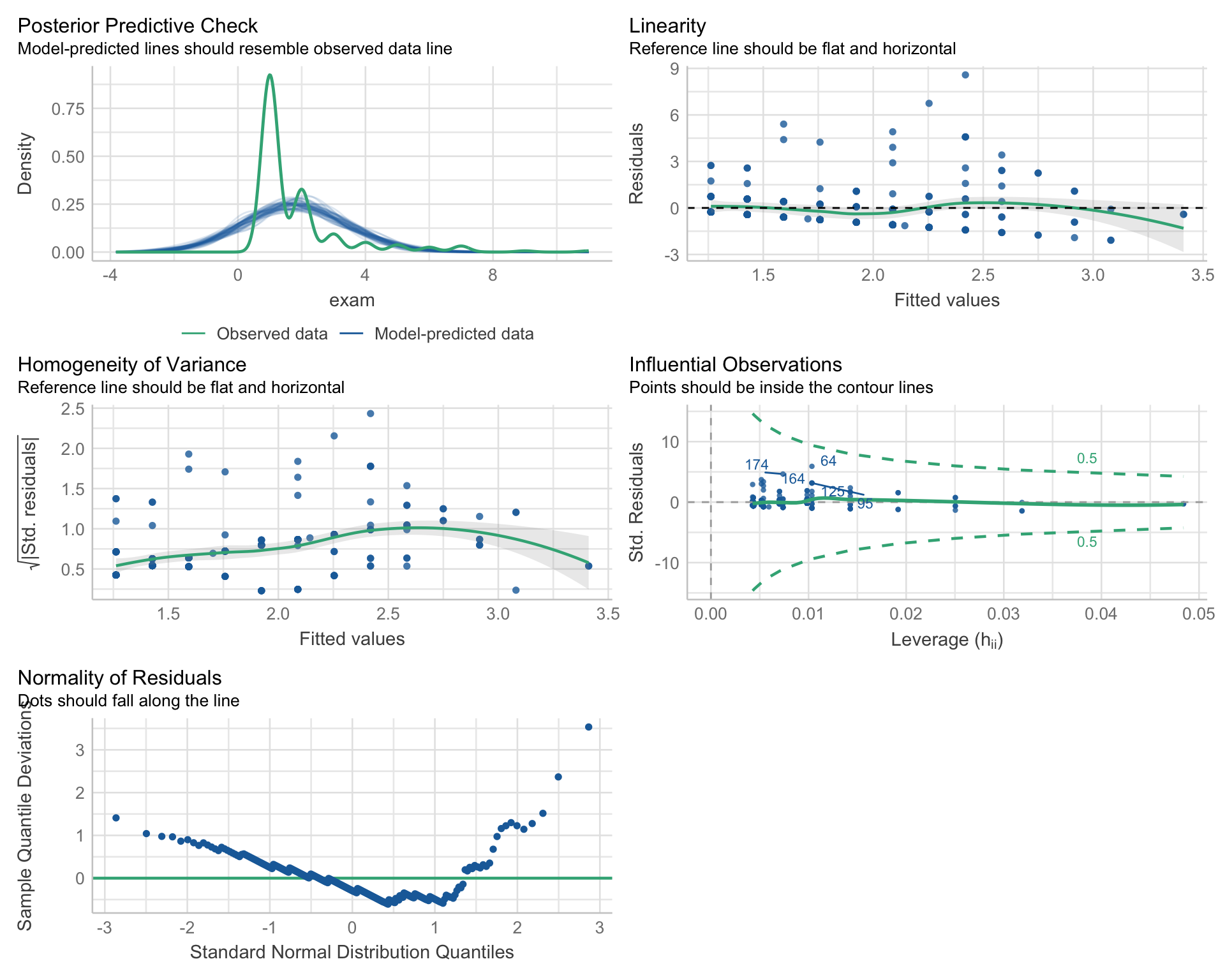
X -> Y
Warning: Non-normality of residuals detected (p < .001).
Warning: Heteroscedasticity (non-constant error variance) detected (p < .001).
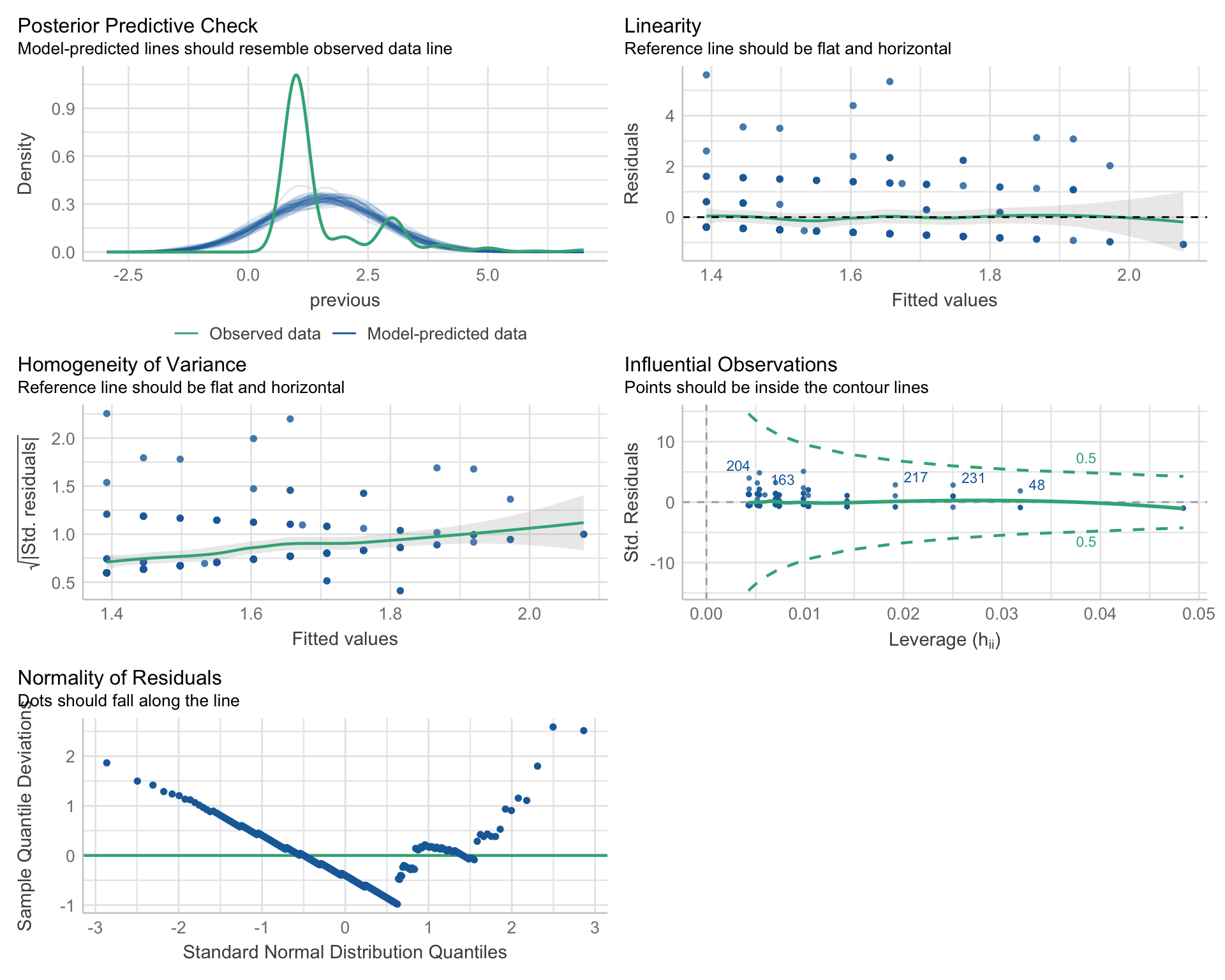
X -> M
Warning: Non-normality of residuals detected (p < .001).
Warning: Heteroscedasticity (non-constant error variance) detected (p = 0.037).
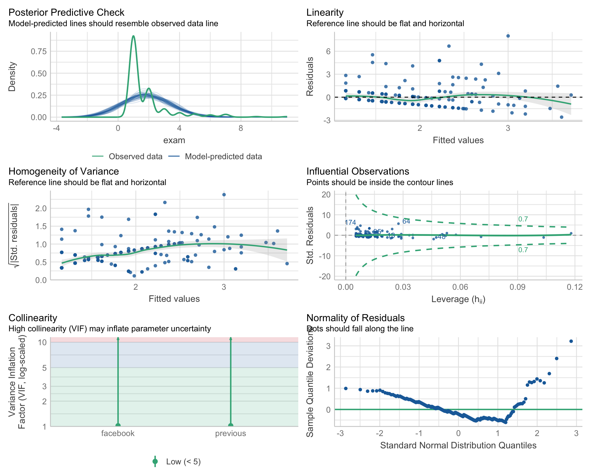
X + M -> Y
Warning: Non-normality of residuals detected (p < .001).
Warning: Heteroscedasticity (non-constant error variance) detected (p < .001).

Complex Mediation Models

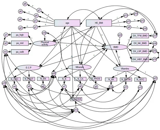
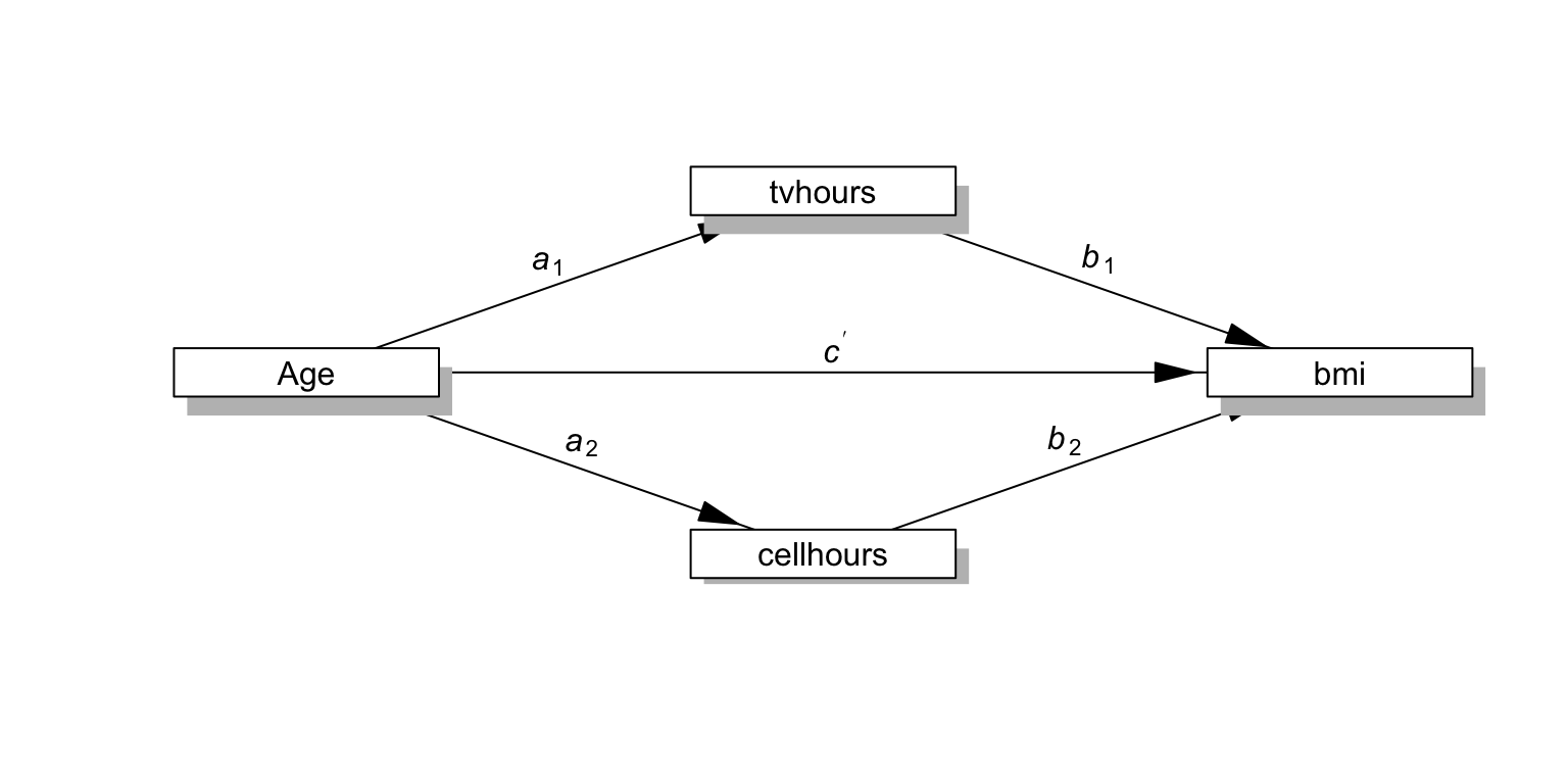
Multiple mediator model

Test the influence of multiple mediator
Specific indirect effect
- X -> M_1 -> Y
- X -> M_2 -> Y
Total indirect effect
- Overall influence of mediators
Can determine which one has a stronger influence

Lavaan

Similar to popular MPlus software, but free!
~ regression; * labels; := define variables

library(lavaan)
multipleMediation <- '
bmi ~ b1 * tvhours + b2 * cellhours + cp * age
tvhours ~ a1 * age
cellhours ~ a2 * age
# Fit indirect 1
indirect1 := a1 * b1
# Fit indirect 2
indirect2 := a2 * b2
# total
total := cp + (a1 * b1) + (a2 * b2)
total_indirect := (a1 * b1) + (a2 * b2)
#test if size of med are different
med_diff := indirect1 - indirect2
#prob mediated
##prop_indirect1
prop_med_1 := indirect1 / (indirect1+cp)
##prop_indirect2
prop_med_2 := indirect2 / (indirect2+cp)
prop_med := total_indirect /(total_indirect+cp)
'
fit <- sem(model = multipleMediation, data = weight_behavior, se = "bootstrap",  bootstrap = 500)

Lavaan summary

summary(fit, ci=TRUE, rsquare=TRUE) # output with 95% bootstrapped cis and rsqaure

lavaan 0.6.17 ended normally after 8 iterations

  Estimator                                         ML
  Optimization method                           NLMINB
  Number of model parameters                         8

  Number of observations                           543

Model Test User Model:
                                                      
  Test statistic                                44.446
  Degrees of freedom                                 1
  P-value (Chi-square)                           0.000

Parameter Estimates:

  Standard errors                            Bootstrap
  Number of requested bootstrap draws              500
  Number of successful bootstrap draws             500

Regressions:
                   Estimate  Std.Err  z-value  P(>|z|) ci.lower ci.upper
  bmi ~                                                                 
    tvhours   (b1)    0.120    0.126    0.947    0.343   -0.145    0.361
    cellhours (b2)    0.217    0.132    1.647    0.100   -0.034    0.470
    age       (cp)    0.026    0.132    0.194    0.846   -0.292    0.227
  tvhours ~                                                             
    age       (a1)    0.017    0.047    0.364    0.716   -0.074    0.129
  cellhours ~                                                           
    age       (a2)    0.041    0.065    0.627    0.530   -0.033    0.226

Variances:
                   Estimate  Std.Err  z-value  P(>|z|) ci.lower ci.upper
   .bmi              15.273    1.620    9.425    0.000   12.209   18.787
   .tvhours           1.883    0.074   25.492    0.000    1.747    2.027
   .cellhours         1.512    0.087   17.340    0.000    1.329    1.666

R-Square:
                   Estimate
    bmi               0.007
    tvhours           0.000
    cellhours         0.002

Defined Parameters:
                   Estimate  Std.Err  z-value  P(>|z|) ci.lower ci.upper
    indirect1         0.002    0.009    0.235    0.814   -0.012    0.025
    indirect2         0.009    0.017    0.526    0.599   -0.009    0.061
    total             0.037    0.130    0.282    0.778   -0.277    0.247
    total_indirect    0.011    0.019    0.569    0.569   -0.013    0.066
    med_diff         -0.007    0.019   -0.362    0.717   -0.061    0.021
    prop_med_1        0.074    2.087    0.036    0.972   -0.816    0.884
    prop_med_2        0.257    1.464    0.176    0.861   -1.845    1.788
    prop_med          0.299   25.095    0.012    0.990   -2.038    2.228

Lavaan summary

semoutput https://dr-jt.github.io/semoutput/

 semoutput::sem_paths(fit)

Predictor	DV	Unstandardized		Standardized
Regression Paths
Predictor	DV	b	95% CI	β	95% CI	sig	SE	z	p
age	bmi	0.026	−0.292 — 0.227	0.008	−0.074 — 0.090		0.042	0.195	0.846
cellhours	bmi	0.217	−0.034 — 0.470	0.068	−0.013 — 0.149		0.041	1.649	0.099
tvhours	bmi	0.120	−0.145 — 0.361	0.042	−0.044 — 0.128		0.044	0.951	0.342
age	cellhours	0.041	−0.033 — 0.226	0.041	−0.088 — 0.171		0.066	0.629	0.529
a1*b1	indirect1	0.002	−0.012 — 0.025	0.001	−0.003 — 0.004		0.002	0.337	0.736
a2*b2	indirect2	0.009	−0.009 — 0.061	0.003	−0.006 — 0.012		0.005	0.610	0.542
indirect1-indirect2	med_diff	−0.007	−0.061 — 0.021	−0.002	−0.012 — 0.007		0.005	−0.444	0.657
total_indirect/(total_indirect+cp)	prop_med	0.299	−2.038 — 2.228	0.299	−2.010 — 2.607		1.178	0.254	0.800
indirect1/(indirect1+cp)	prop_med_1	0.074	−0.816 — 0.884	0.074	−0.729 — 0.878		0.410	0.181	0.856
indirect2/(indirect2+cp)	prop_med_2	0.257	−1.845 — 1.788	0.257	−1.884 — 2.398		1.092	0.235	0.814
cp+(a1b1)+(a2b2)	total	0.037	−0.277 — 0.247	0.012	−0.069 — 0.092		0.041	0.282	0.778
(a1b1)+(a2b2)	total_indirect	0.011	−0.013 — 0.066	0.003	−0.007 — 0.014		0.005	0.675	0.499
age	tvhours	0.017	−0.074 — 0.129	0.016	−0.069 — 0.100		0.043	0.364	0.716
* p < .05; p < .01; * p < .001

Lavaan summary

easystats provides nice summary function

parameters::model_parameters(fit)

# Regression

Link                 | Coefficient |   SE |        95% CI |    z |     p
------------------------------------------------------------------------
bmi ~ tvhours (b1)   |        0.12 | 0.13 | [-0.14, 0.36] | 0.95 | 0.343
bmi ~ cellhours (b2) |        0.22 | 0.13 | [-0.03, 0.47] | 1.65 | 0.100
bmi ~ age (cp)       |        0.03 | 0.13 | [-0.29, 0.23] | 0.19 | 0.846
tvhours ~ age (a1)   |        0.02 | 0.05 | [-0.07, 0.13] | 0.36 | 0.716
cellhours ~ age (a2) |        0.04 | 0.07 | [-0.03, 0.23] | 0.63 | 0.530

# Defined

To               | Coefficient |       SE |        95% CI |     z |     p
-------------------------------------------------------------------------
(indirect1)      |    2.06e-03 | 8.77e-03 | [-0.01, 0.03] |  0.24 | 0.814
(indirect2)      |    8.89e-03 |     0.02 | [-0.01, 0.06] |  0.53 | 0.599
(total)          |        0.04 |     0.13 | [-0.28, 0.25] |  0.28 | 0.778
(total_indirect) |        0.01 |     0.02 | [-0.01, 0.07] |  0.57 | 0.569
(med_diff)       |   -6.82e-03 |     0.02 | [-0.06, 0.02] | -0.36 | 0.717
(prop_med_1)     |        0.07 |     2.09 | [-0.82, 0.88] |  0.04 | 0.972
(prop_med_2)     |        0.26 |     1.46 | [-1.85, 1.79] |  0.18 | 0.861
(prop_med)       |        0.30 |    25.10 | [-2.04, 2.23] |  0.01 | 0.990

Lavaan Visualization

library(tidySEM)# plot models from lavaan

parallel_map <- tidySEM::get_layout("", "tvhours", "", "age", "", "bmi", "", "cellhours",
                                    "", rows = 3)
tidySEM::graph_sem(model=fit, layout=parallel_map)

Lavaan Practice

Fit our simple facebook mediation model using Lavaan

Lavaan Practice

Look at that! Same results as before

Predictor	DV	Unstandardized		Standardized
Regression Paths
Predictor	DV	b	95% CI	β	95% CI	sig	SE	z	p
facebook	exam	−0.606	−0.921 — −0.351	−0.292	−0.398 — −0.185	***	0.054	−5.361	<0.001
previous	exam	0.260	0.081 — 0.497	0.189	0.043 — 0.334	*	0.074	2.545	0.011
a*b	indirect	−0.055	−0.150 — 0.002	−0.026	−0.059 — 0.007		0.017	−1.565	0.118
facebook	previous	−0.211	−0.429 — 0.007	−0.139	−0.281 — 0.003		0.072	−1.923	0.055
cp+(a*b)	total	−0.661	−1.002 — −0.402	−0.318	−0.425 — −0.211	***	0.055	−5.816	<0.001
* p < .05; p < .01; * p < .001

Within-participant mediation

Mediation when X is a within-subject variable
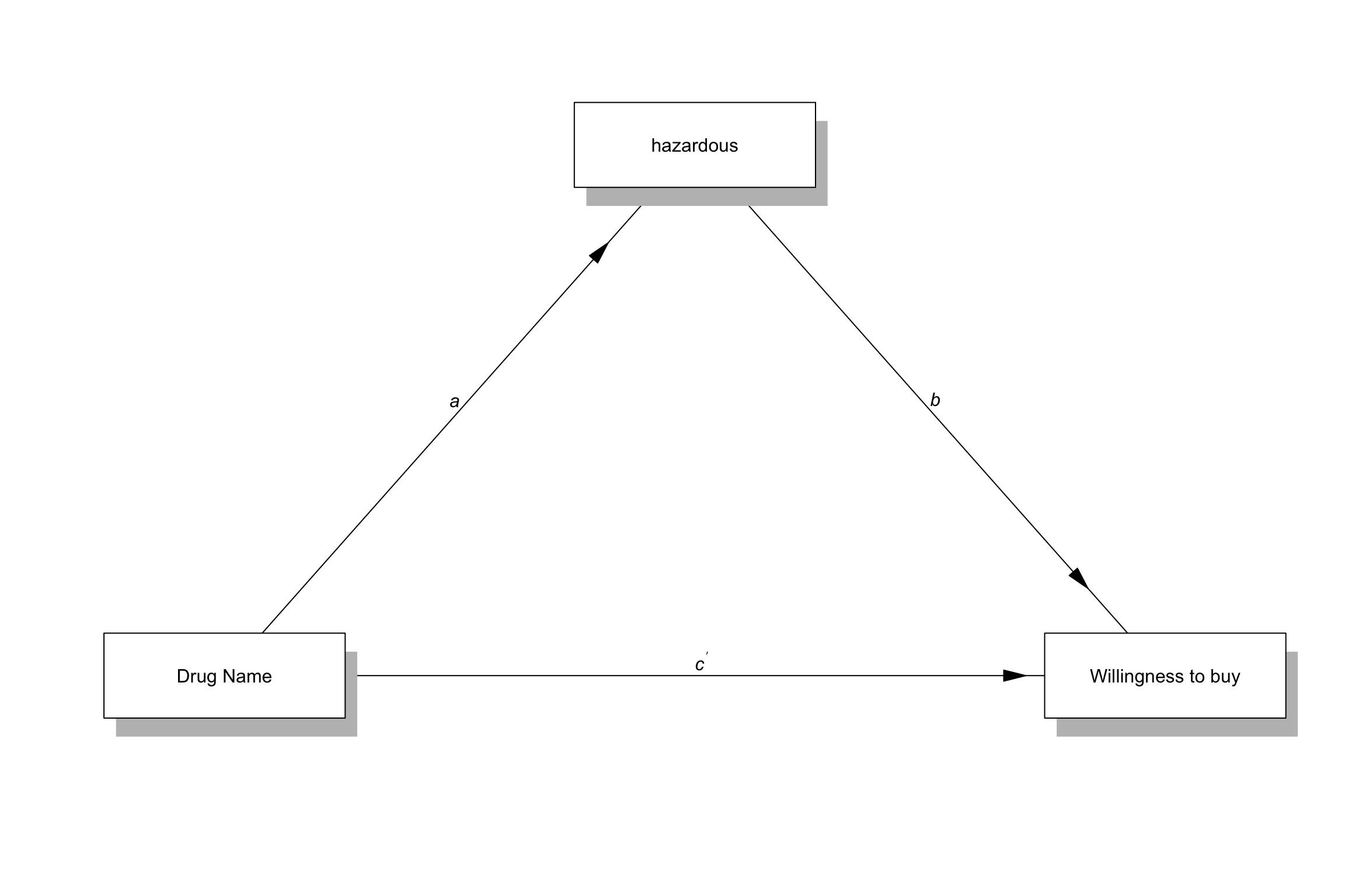
Dohle and Siegrist (2014, Exp 1)
- Interested in the effect of name complexity on buying drugs
  - The specific hypothesis is that complex drug names are perceived as more hazardous, which makes someone less likely to buy the drug

Within-participant mediation

\[ Y_{2i} - Y_{1i} = c_{11} \]

with \(Y2_i\)−\(Y1_i\) the difference score between DV conditions for the outcome variable for the ith observation

\[ M_{2i}-M_{1i} = a_{21} \]

with \(M_{2i}\)−\(M1_{1i}\) the difference score between DV conditions for the mediator variable for the ith observation,

\[Y_{2i} - Y_{1i} = c'_{31} + b_{32}(M_{2i} - M_{1i}) + d_{33}[0.5(M_{1i} + M_{2i}) - 0.5(\overline{M_{1} + M_{2}})]\]

Where we have the direct path, mediator diff and mean_diff

Within-participant mediation

data <- JSmediation::dohle_siegrist

within_mdt <- mdt_within(data=data, IV=name, DV= willingness, M=hazardousness,grouping=participant)

Note

Montoya, A. K., & Hayes, A. F. (2017). Two-condition within-participant statistical mediation analysis: A path-analytic framework. Psychological Methods, 22(1), 6-27. doi: 10.1037/met0000086

Within-participant indirect effect

model_fit_with_index <- add_index(within_mdt)
model_fit_with_index

Test of mediation (within-participant_mediation)
==============================================

Variables:

- IV: name (difference: simple - complex) 
- DV: willingness 
- M: hazardousness 

Paths:

====  ==============  =====  ======================
Path  Point estimate     SE  APA                   
====  ==============  =====  ======================
a             -0.800  0.258  t(21) = 3.10, p = .005
b             -0.598  0.113  t(19) = 5.29, p < .001
c              0.564  0.193  t(21) = 2.92, p = .008
c'             0.085  0.158  t(19) = 0.54, p = .596
====  ==============  =====  ======================

Indirect effect index:

- type: Within-participant indirect effect 
- point estimate: 0.479 
- confidence interval:
  - method: Monte Carlo (5000 iterations)
  - level: 0.05 
  - CI: [0.163; 0.865]

Fitted models:

- 1 -> DV_diff 
- 1 -> M_diff 
- 1 + M_diff + M_mean -> DV_diff

Summary: Mediation

What it is: A method for testing hypotheses about why and how x predicts y
When you use it:
- Whenever you would start using words like “because” in your introduction section
Best approach*:
- Bootstrapping

Write-up: Mediation

a, b paths
Direct effect (c’)
Total effect (c)
Indirect effect
How did you test indirect effect
- Sobel test or Bootstrapping (# bootstrapped samples)
Proportion mediated

Figure of path diagram
- Create in PPT 😱
- Use DiagrammeR

Write up: Multiple mediators

Include all indirect effects
Total indirect effect
Proportion mediated

Resources

Other R packages
- mediation (ordinal or binary outcomes)
- manymome
- processR
- bmlm (Bayesian)
- bayestestR (mediation function)

Wednesday and next week

Mediation lab

Path modeling/SEM (Renata and Brooke)