Introduction to Structural Equation Modeling in R

Princeton University

Jason Geller, PH.D.

2024-04-14

Today

• What is structural equation modeling (SEM)?

  • Path models

  • Important terminology

• How to do it in R

  • Specification

  • Identification

  • Estimation

  • Model fit & indices

  • Modification indices

  • Reporting

Packages

library(easystats)
library(tidyverse)
library(lavaan)
library(tidygraph)
library(processR)
library(knitr)

options(scipen=999)

• Follow along:https://github.com/jgeller112/PSY504-Advanced-Stats-S24/blob/main/slides/11-SEM/sem_intro_1.qmd

Structural equation modeling

• A broad range of of techniques and frameworks

  • Not a single technique

    • Integration of:

      • Path analysis

      • Confirmatory factor analysis

• Used to test and quantify theories

• Model variables that exist (manifest) and those that don’t technically exist (latent factors)

Structural equation modeling

• You already know how to do it!

  • It is regression on steroids

  • Model many relationships at once, rather than run single regressions

Path analysis

• A method for testing any possible relationship between measured variables

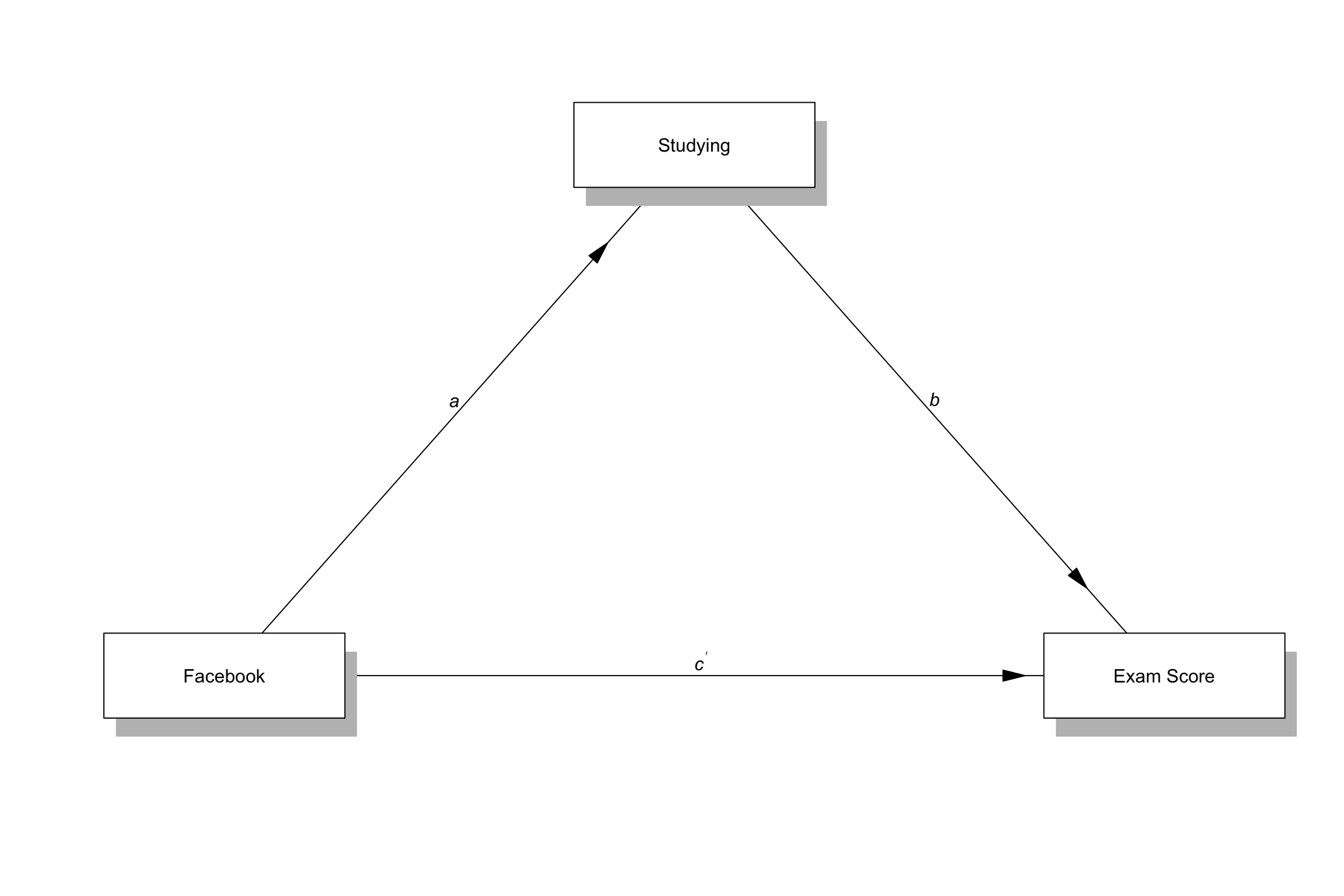
Terminology

Exogenous vs. endogenous variables

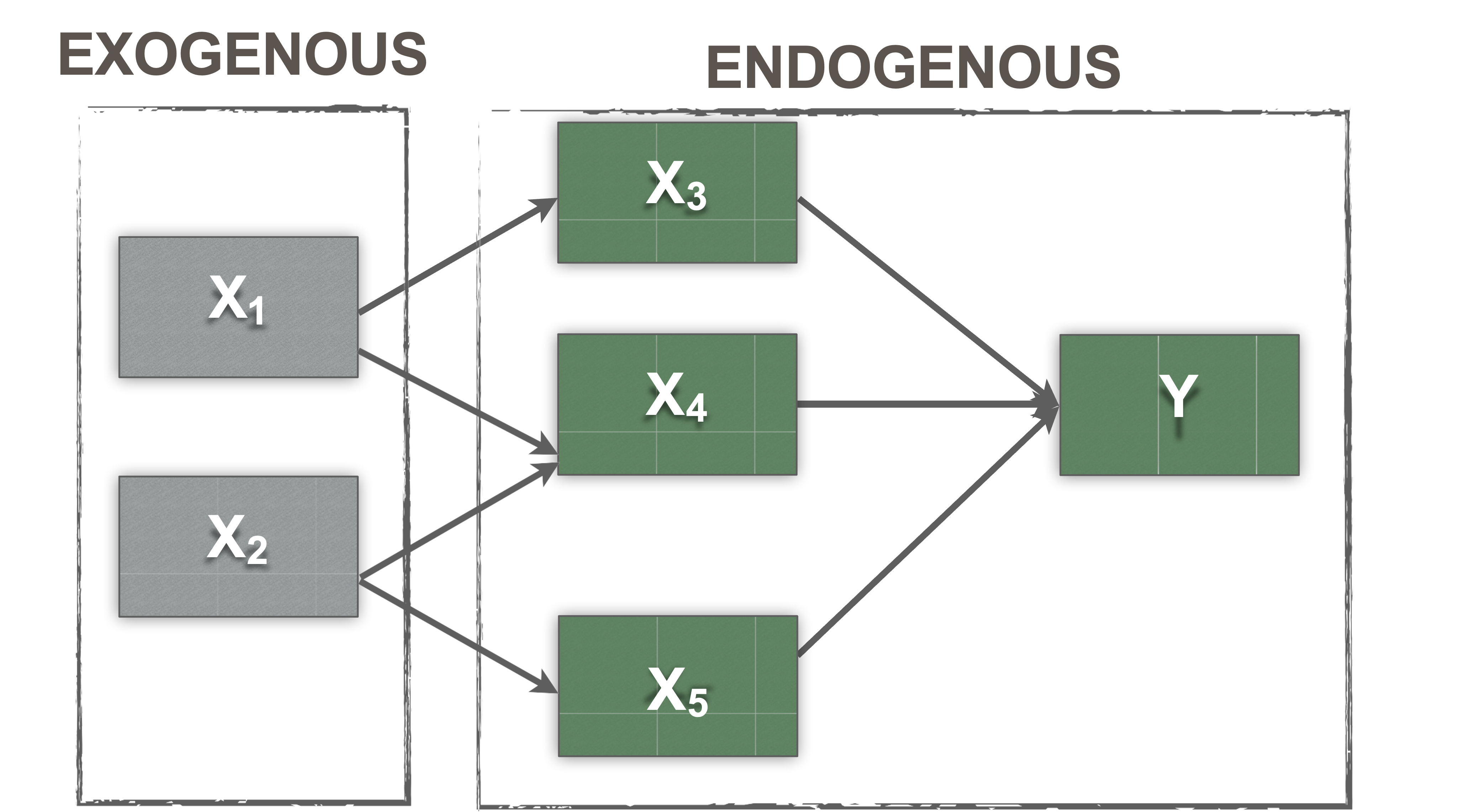
• Exogenous
  • These are synonymous with independent variables
  • You can find these in a model where the arrow is leaving the variable
    • They are thought to be the cause of something
  • Have variance
  • Covary with other exogenous variables (default)

Exogenous vs. endogenous variables

• Endogenous
  • These are synonymous with dependent variables
  • They are caused by the exogenous variables
  • In a model diagram, the arrow will be coming into the variable
  • Have error terms (disturbances)

Endogenous vs. Exogenous

• TL;DR

  • Exogenous: no arrows pointed at it

  • Endogenous: arrows pointed at it

Manifest variables vs. latent variables

• Manifest or observed variables

  • Represented by squares ❏

  • Measured from participants, business data, or other sources

  • While most measured variables are continuous, you can use categorical and ordered measures as well

Manifest variables vs. latent variables

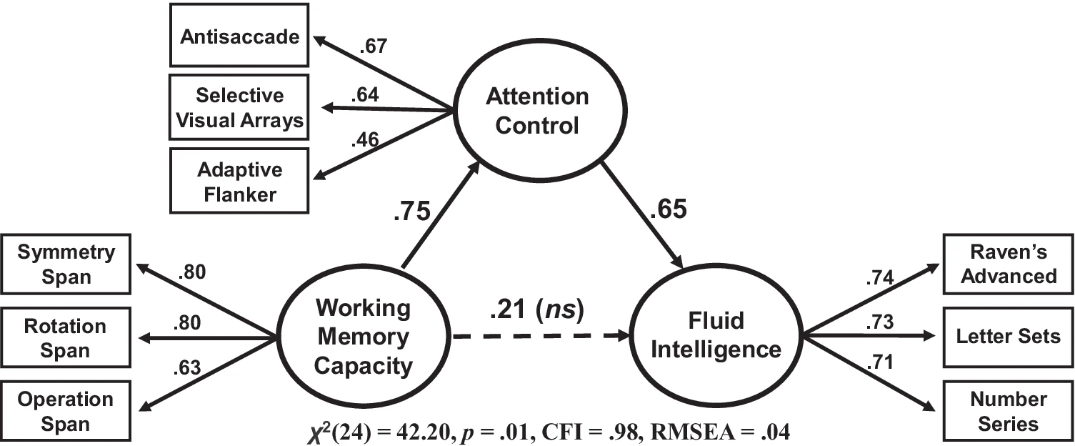
• Latent variables

  • Represented by circles ◯

  • Abstract phenomena you are trying to model

  • Are not represented by a number in the dataset

  • Linked to the measured variables

  • Represented indirectly by those variables

Remember

• Y~X + Residual

• Here that is Endogenous ~ Exogenous + disturbance

Variances, covariances, and disturbances

• Variance

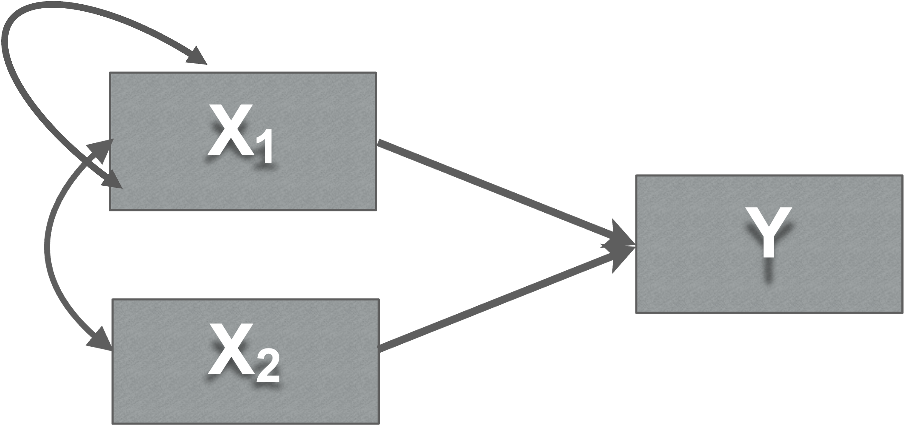
• Double headed arrows
  • To itself

Variances, covariances, and disturbances

• Covariance paths

• Double headed arrows (Covariance paths)
• Exogenous variables may be correlated with each other, but not always…

Covariance meaning

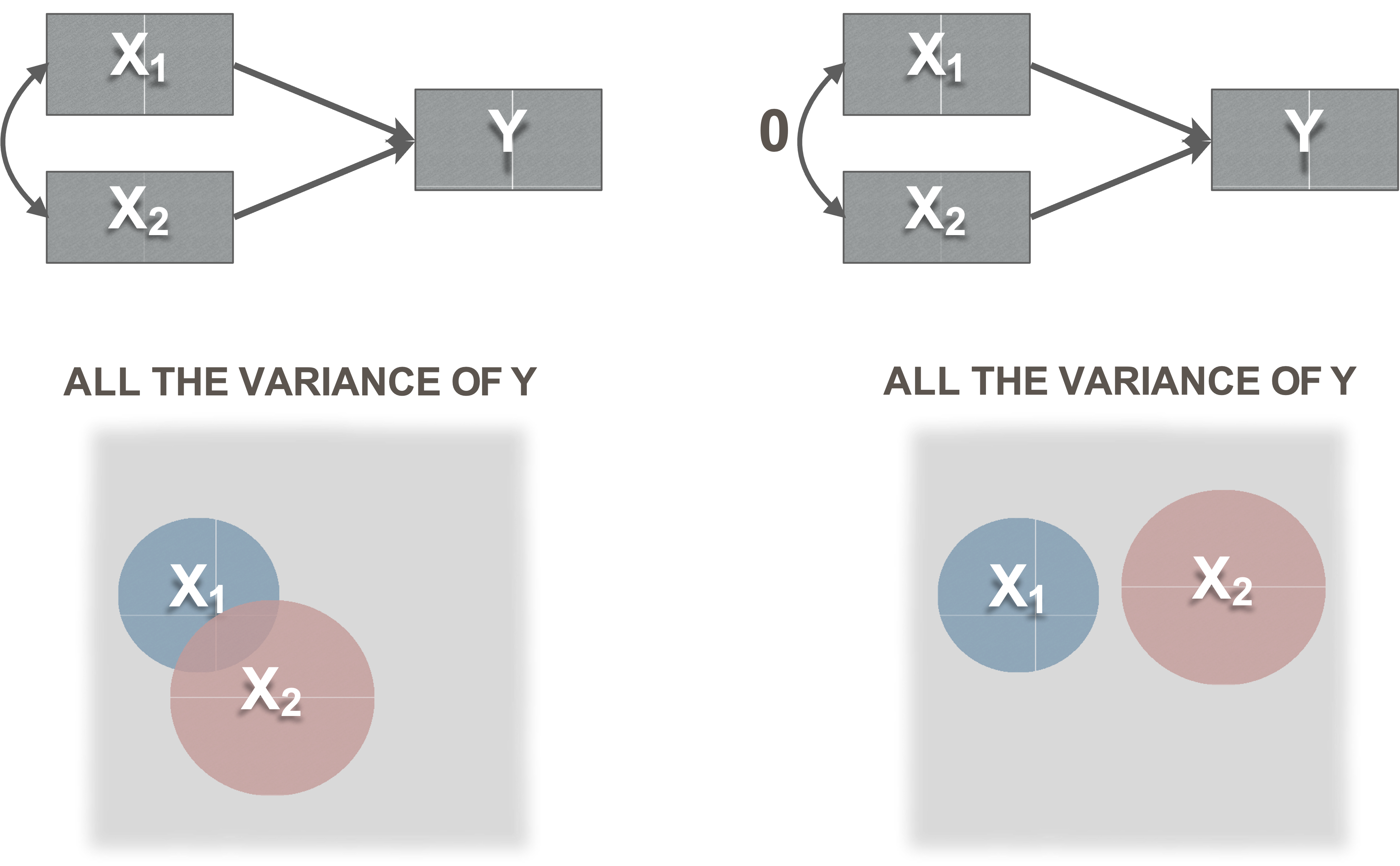
Variances, covariances, and disturbances

• Disturbances

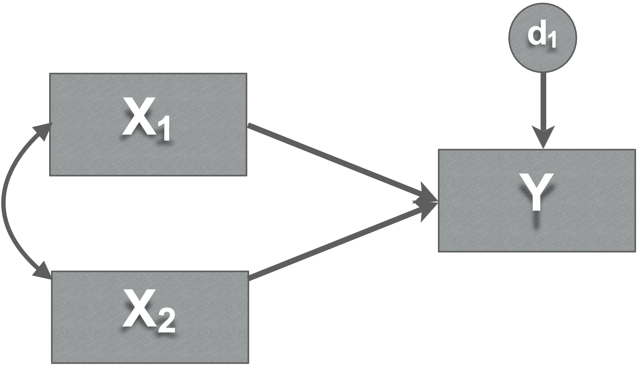
• Represent the influence of factors not included in model

• error in your prediction of each endogenous variable

• Every endogenous variable has a disturbance

SEM models

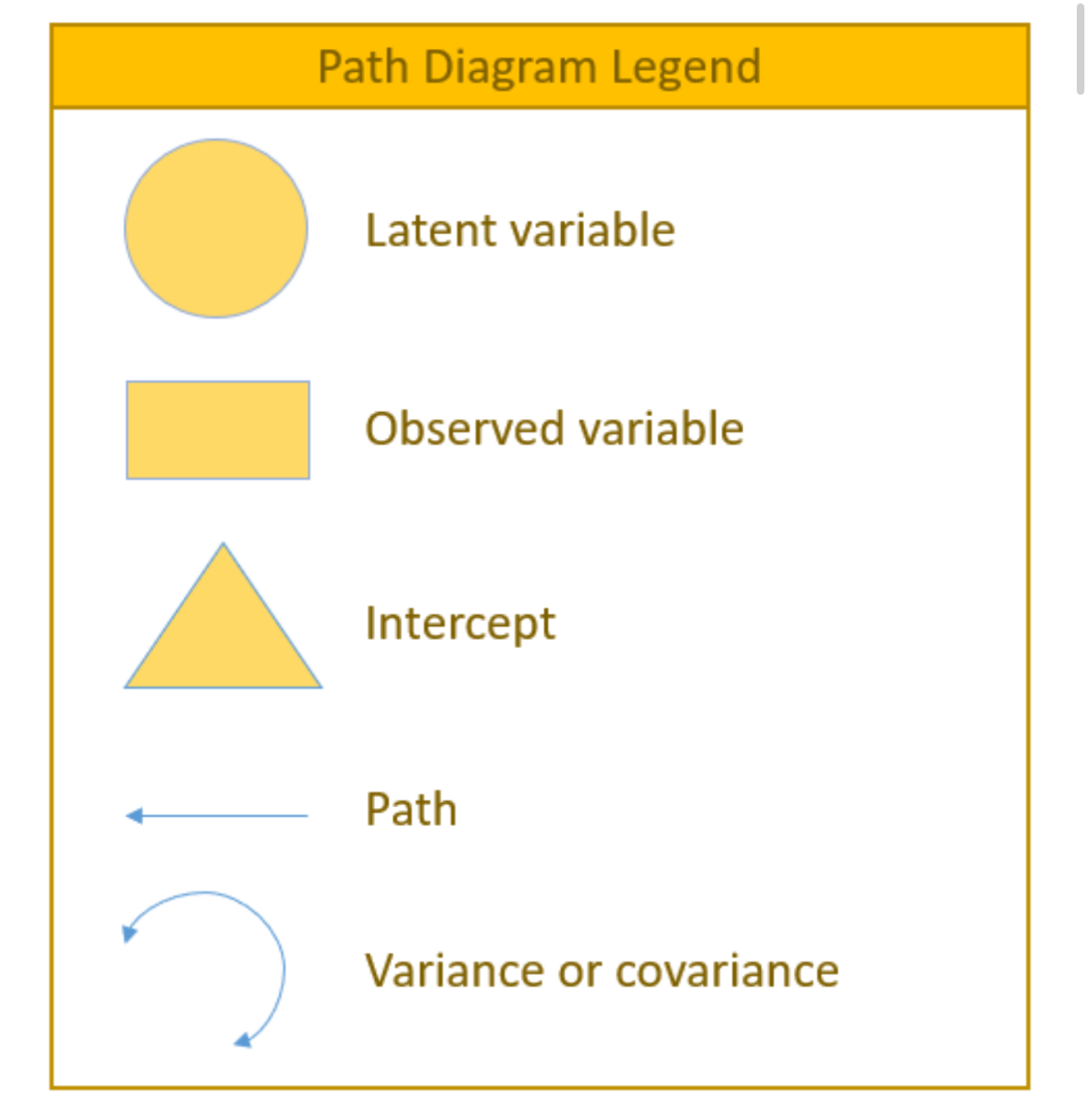
• Straight arrows are “causal” or directional

  • Non-standardized solution -> these are your b or slope values
  • Standardized solution -> these are your beta values

• Curved arrows are non-directional

  • Non-standardized -> covariance
  • Standardized -> correlation

Cheat sheet

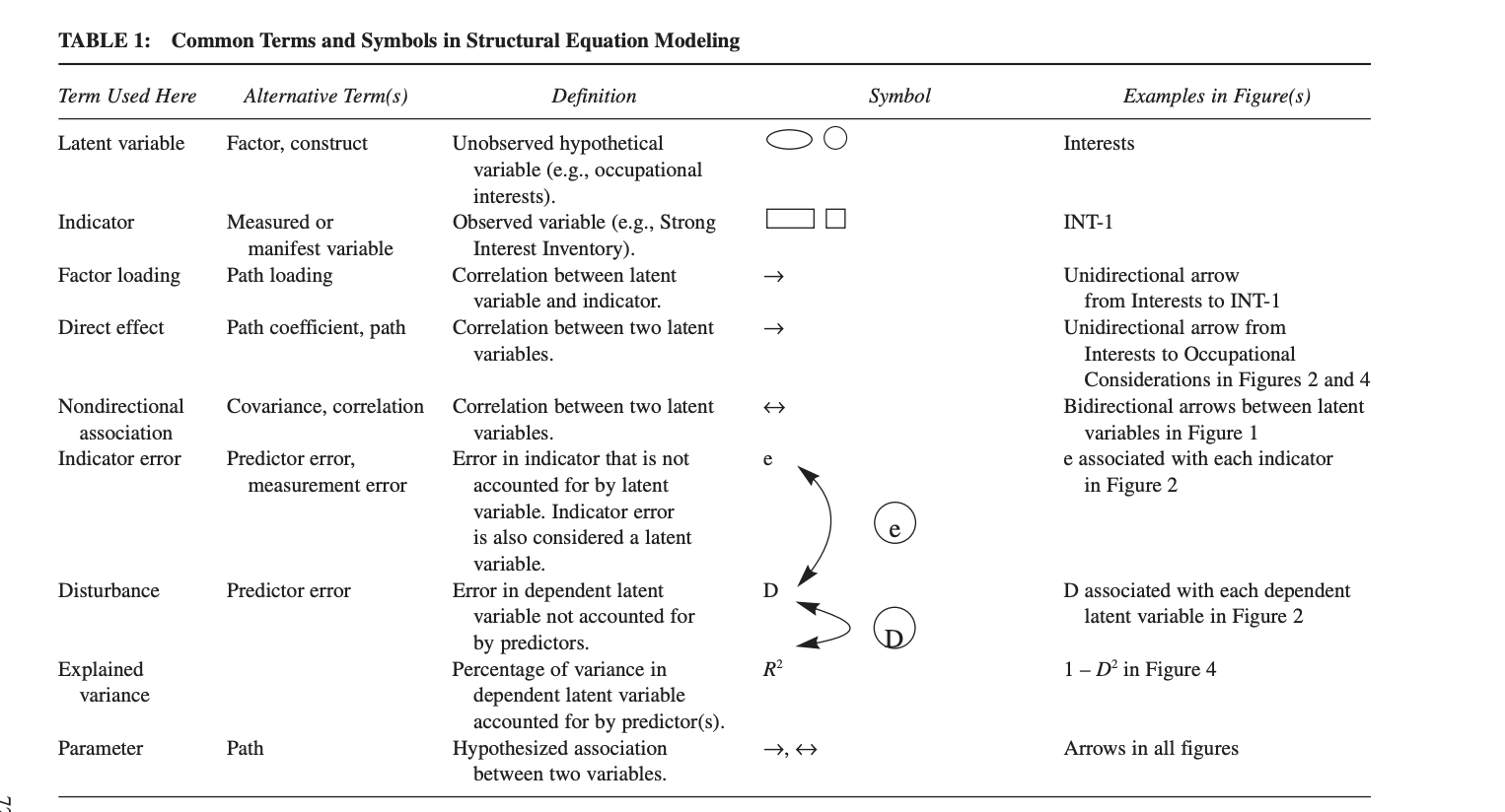
• Also here: https://davidakenny.net/cm/basics.htm

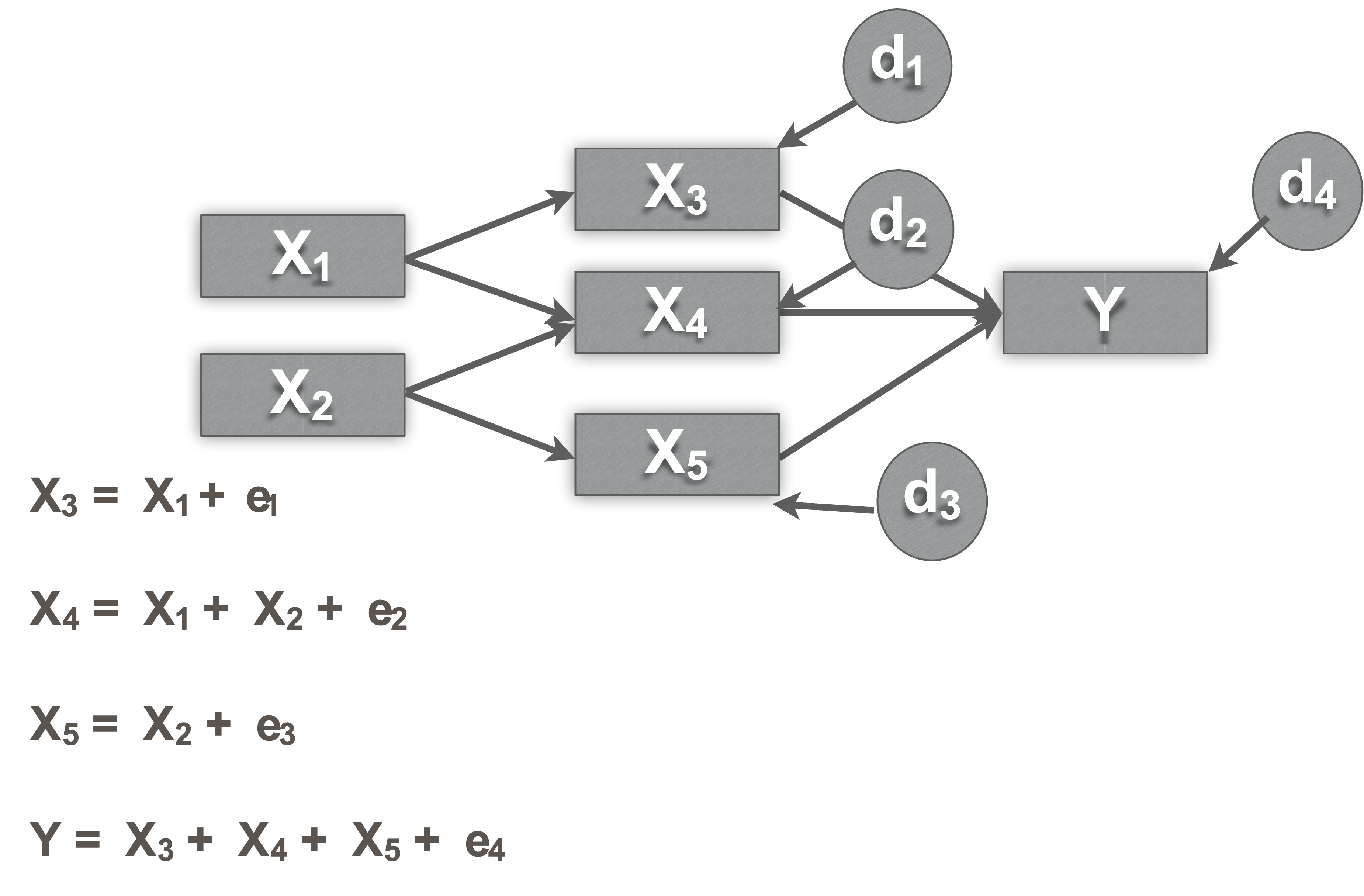
Why is it just regression?

Each endogenous variable is regressed on all exogenous variables that are connected in the chain that leads directly to it

Identification

Model identification

• You cannot test all models

  • Unique solution

• If not identified, cannot analyze model

• How is this determined?

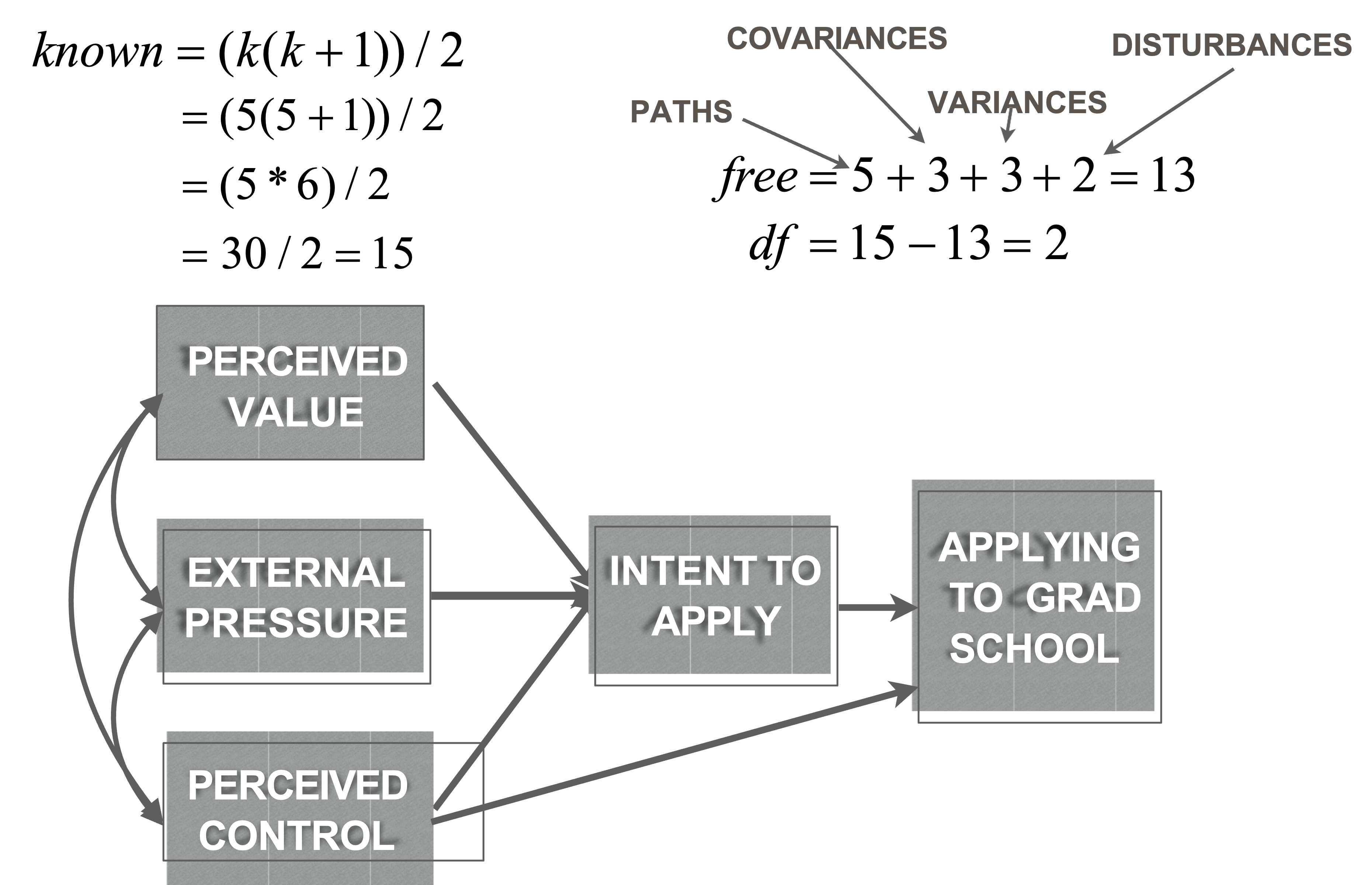
Minimum condition of identification

• There must be at least as many known values in the model as there are free parameters

• Free parameters:

  • All regression paths, all covariances, all variances, and all disturbances in the model

• Knowns:

  \[\frac{(K (K+1))}{2}\]- where k is number of measured variables

Model identification

• We can tell model is identified by calculating model DFs

  • Additional pathways you can estimate

• Model DF = (known values) - (free parameters)

Model identification

• If model DF >=1 you can analyze model

  • Over-identified

• DF = 0 (saturated)

  • You can still analyze the model

    • But:

      • Fits data perfectly

      • No fit indices

    • Multiple regressions are just-identified model

• DF < 0

  • Under-identified

  • Cant analyze our model

Identification

• Just-identified - mathematical analogy

  • 10=2x+y

  • 2 = x-y

    • 2 knows and 2 unknowns

    • One set of values that can solve the equation

• Can’t test other models

• Under-identified - mathematical analogy

  • 10 = x+ y

    • One known value and 2 unknowns (x,y)

    • There are infinite number of solutions

    • No way to derive a solution

Identification

• Over-identified - mathematical analogy

  • 10=2x+y

  • 2 = x-y

  • 5 = x + 2y

• Several possible approximate solutions to solve all 3 equations
• Several unique but imperfect solutions means multiple models can be tested or compared
• You can’t evaluate fit without alternatives

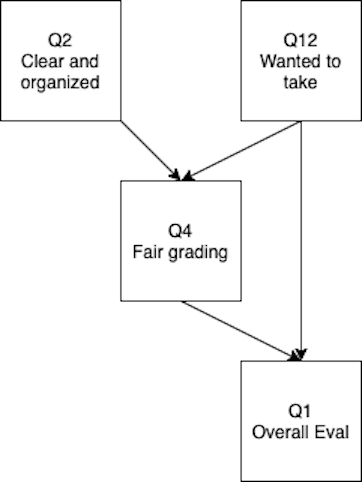
Estimate DFs

• Let’s play a game

03:00

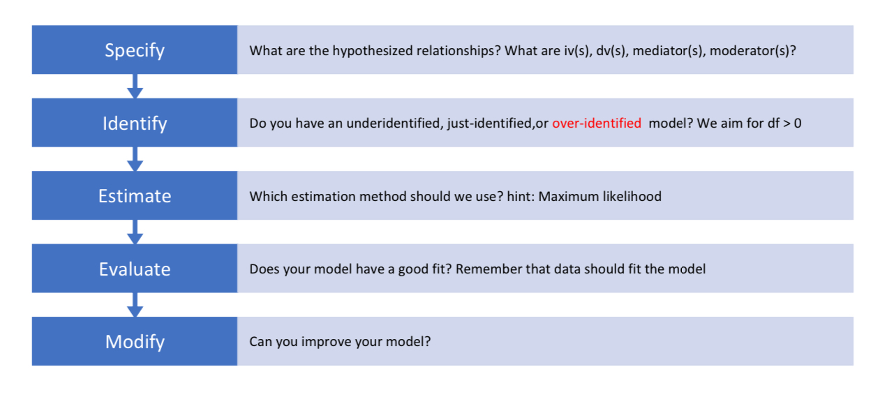
SEM steps

Example data (Ingram et al., 2000)

• What makes someone apply to graduate school?

• Endogenous

  • Intent to apply (intent.to.apply)
  • Apply (application.behaviour)

• Exogenous:

  • Perceived value (perceived.value)
  • External pressure (external.pressure)
  • Perceived control over admission (perceived.control)

grad <- read.csv("https://raw.githubusercontent.com/jgeller112/psy504-advanced-stats/main/slides/SEM/data/graduate.school.csv") %>% 
  dplyr::select(-job.opportunities)

Model specification

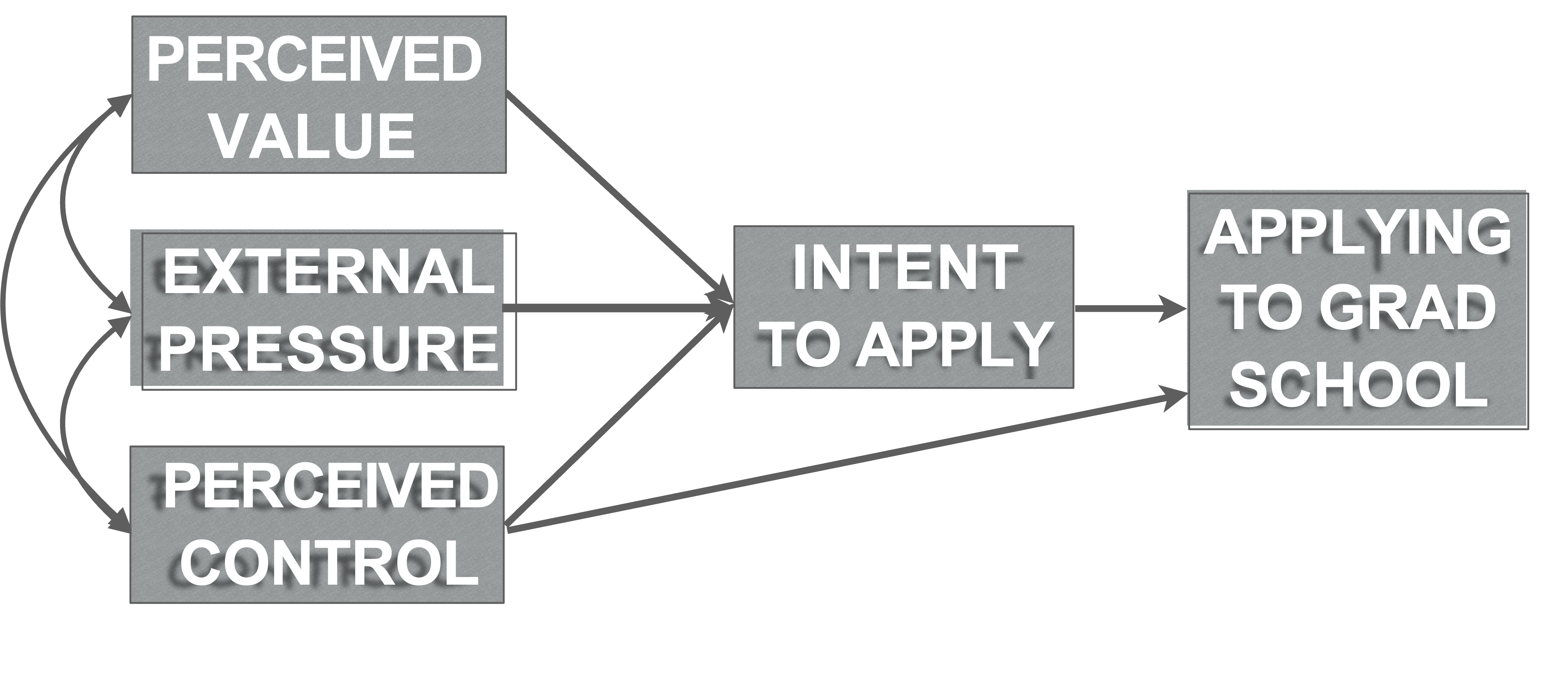
• Theory of planned behavior

Data screening

correlation::correlation(grad, redundant = FALSE) %>% plot()

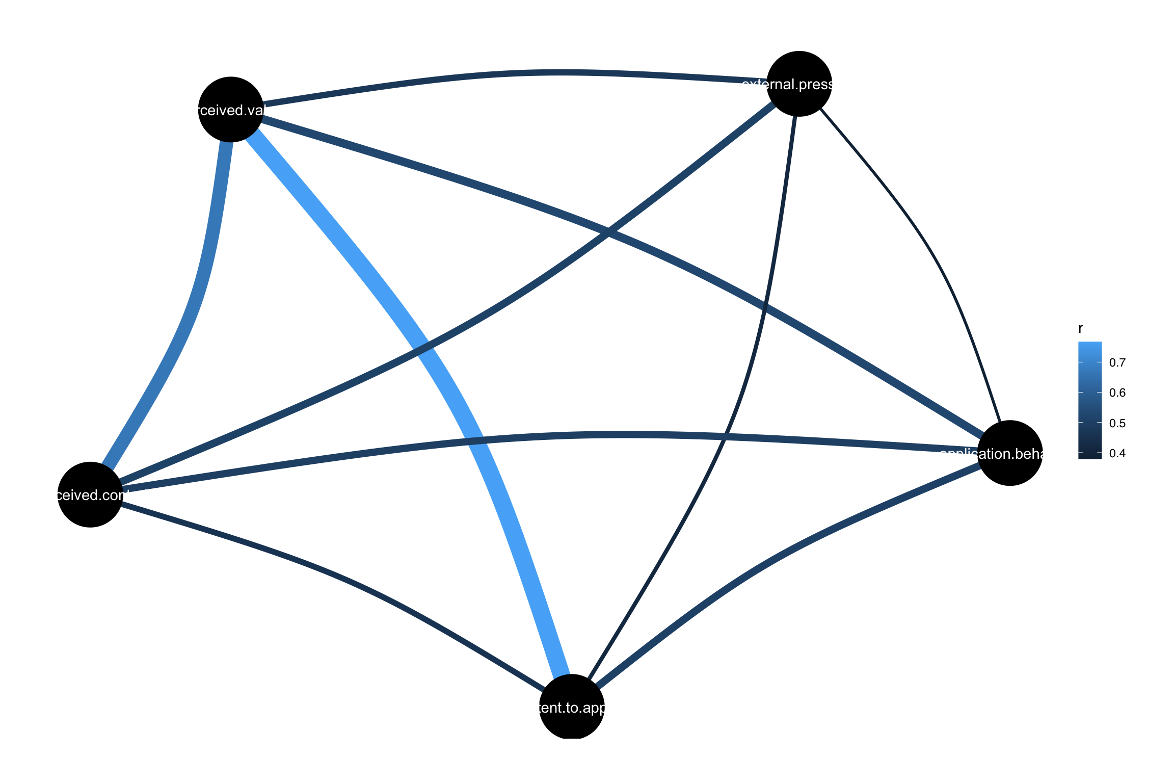
Identification

Run SEM in R

library(lavaan)
library(semPlot)

• Declare equations for every endogenous variable in your model

  • `~` indicates a regression

• Declare indirect and covariances

  • := declare a variable

  • * name of variable

  • ~~ indicates a covariance/correlation

  • =~ latent factor

Run SEM in R

grad_model = '
intent.to.apply~a*perceived.value+b*external.pressure+c*perceived.control 

    application.behaviour~d*intent.to.apply+ e*perceived.control 
    #indirect
    value.through.intent:=a*d
    #indirect
    pressure.through.intent:=b*d 
    #indirect
    control.through.intent:=c*d 

 perceived.control ~~ perceived.value # These are covariance paths
  perceived.control ~~ external.pressure # These are covariance paths
  external.pressure ~~ perceived.value # These are covariance paths
'
fit <- sem(grad_model, se="bootstrap", bootstrap=5000,  data=grad)

Model fit

• SEM compares the observed covariance matrix to predicted or model-based covariance matrix

  • We want to know if our theoretical model fits the data

  • Good fit means we’ve captured the bulk of relations between variables in our model and there is not much covariance left over

    • We didn’t miss anything

• This means we compare the relationships we’ve modeled to all possible relationships

Model fit

Fit measure	Name	Cutoff
\(\chi^2\)*	Chi-square	p > .05
(A)GFI	Adjusted Goodness of Fit	AGFI ≥ .90
TLI*	Tucker Lewis Index	TLI ≥ .95
CFI*	Comparative Fit Index	CFI ≥ .90
RMSEA*	Root Mean Square Error of Approximation	RMSEA < .08
(S)RMR*	Standardized Root Mean Square Residual	SRMR < .08
AVE (in CFAs)	Average Value Explained	AVE > .5

• Common to use \(\chi^2\), RMSEA, SRMR, CFI

Note

Hu, L.-t., & Bentler, P. M. (1999). Cutoff criteria for fit indexes in covariance structure analysis: Conventional criteria versus new alternatives. Structural Equation Modeling, 6(1), 1–55. https://doi.org/10.1080/10705519909540118

Model fit

• • Absolute fit (measures how well data fits specified model)

    • \(\chi^2\) (sensitive to sample size)

    • SRMR

      • Standardized difference between the sample covariance matrix and hypothesized covariance matrix

  • Badness of fit

    • RMSEA

      • Measures how much worse the data fits the model from the just identified model

  • Relative goodness of fit

    • CFI or TLI

      • Measures how much better the model fits than the null model (all paths=0)

Run SEM

fit <- sem(grad_model, se="bootstrap", bootstrap=5000, data=grad)

summary(fit, ci=TRUE, 
        standardize=TRUE, # get standardized 
        fit.measures=TRUE) # get fit indices

lavaan 0.6.17 ended normally after 60 iterations

  Estimator                                         ML
  Optimization method                           NLMINB
  Number of model parameters                        13

  Number of observations                            60

Model Test User Model:
                                                      
  Test statistic                                 0.862
  Degrees of freedom                                 2
  P-value (Chi-square)                           0.650

Model Test Baseline Model:

  Test statistic                               136.416
  Degrees of freedom                                10
  P-value                                        0.000

User Model versus Baseline Model:

  Comparative Fit Index (CFI)                    1.000
  Tucker-Lewis Index (TLI)                       1.045

Loglikelihood and Information Criteria:

  Loglikelihood user model (H0)               -993.733
  Loglikelihood unrestricted model (H1)       -993.303
                                                      
  Akaike (AIC)                                2013.467
  Bayesian (BIC)                              2040.693
  Sample-size adjusted Bayesian (SABIC)       1999.805

Root Mean Square Error of Approximation:

  RMSEA                                          0.000
  90 Percent confidence interval - lower         0.000
  90 Percent confidence interval - upper         0.200
  P-value H_0: RMSEA <= 0.050                    0.690
  P-value H_0: RMSEA >= 0.080                    0.257

Standardized Root Mean Square Residual:

  SRMR                                           0.019

Parameter Estimates:

  Standard errors                            Bootstrap
  Number of requested bootstrap draws             5000
  Number of successful bootstrap draws            4998

Regressions:
                          Estimate  Std.Err  z-value  P(>|z|) ci.lower ci.upper
  intent.to.apply ~                                                            
    percevd.vl (a)           0.444    0.058    7.714    0.000    0.323    0.551
    extrnl.prs (b)           0.029    0.035    0.850    0.396   -0.035    0.101
    prcvd.cntr (c)          -0.064    0.059   -1.075    0.282   -0.191    0.042
  application.behaviour ~                                                      
    intnt.t.pp (d)           1.520    0.535    2.840    0.005    0.487    2.593
    prcvd.cntr (e)           0.734    0.303    2.422    0.015    0.249    1.455
   Std.lv  Std.all
                  
    0.444    0.807
    0.029    0.095
   -0.064   -0.126
                  
    1.520    0.350
    0.734    0.336

Covariances:
                       Estimate  Std.Err  z-value  P(>|z|) ci.lower ci.upper
  perceived.value ~~                                                        
    perceivd.cntrl       34.696   10.891    3.186    0.001   16.025   58.051
  external.pressure ~~                                                      
    perceivd.cntrl       46.660   13.080    3.567    0.000   22.627   73.386
  perceived.value ~~                                                        
    external.prssr       39.758   11.894    3.343    0.001   16.815   63.559
   Std.lv  Std.all
                  
   34.696    0.665
                  
   46.660    0.505
                  
   39.758    0.472

Variances:
                   Estimate  Std.Err  z-value  P(>|z|) ci.lower ci.upper
   .intent.to.pply    5.780    0.987    5.855    0.000    3.537    7.384
   .applicatn.bhvr  179.514   27.923    6.429    0.000  118.564  228.012
    perceived.valu   47.616    9.468    5.029    0.000   30.203   67.277
    external.prssr  149.236   22.301    6.692    0.000  105.792  193.454
    perceivd.cntrl   57.154   14.014    4.078    0.000   31.636   85.717
   Std.lv  Std.all
    5.780    0.400
  179.514    0.657
   47.616    1.000
  149.236    1.000
   57.154    1.000

Defined Parameters:
                   Estimate  Std.Err  z-value  P(>|z|) ci.lower ci.upper
    val.thrgh.ntnt    0.675    0.252    2.683    0.007    0.200    1.199
    prssr.thrgh.nt    0.045    0.058    0.768    0.442   -0.055    0.180
    cntrl.thrgh.nt   -0.097    0.111   -0.870    0.384   -0.379    0.056
   Std.lv  Std.all
    0.675    0.282
    0.045    0.033
   -0.097   -0.044

What to report?

• easystats has you covered!

interpret(fit)

    Name      Value Threshold Interpretation
1    GFI 0.99432949      0.95   satisfactory
2   AGFI 0.95747118      0.90   satisfactory
3    NFI 0.99368415      0.90   satisfactory
4   NNFI 1.04502659      0.90   satisfactory
5    CFI 1.00000000      0.90   satisfactory
6  RMSEA 0.00000000      0.05   satisfactory
7   SRMR 0.01902056      0.08   satisfactory
8    RFI 0.96842073      0.90   satisfactory
9   PNFI 0.19873683      0.50           poor
10   IFI 1.00846935      0.90   satisfactory

Reporting Results

suppressWarnings(report_performance(fit))

The model is not significantly different from a baseline model (Chi2(2) = 0.86,
p = 0.650). The GFI (.99 > .95) suggest a satisfactory fit. The PNFI (.20 <
.50) suggests a poor fit., The model is not significantly different from a
baseline model (Chi2(2) = 0.86, p = 0.650). The AGFI (.96 > .90) suggest a
satisfactory fit. The PNFI (.20 < .50) suggests a poor fit., The model is not
significantly different from a baseline model (Chi2(2) = 0.86, p = 0.650). The
NFI (.99 > .90) suggest a satisfactory fit. The PNFI (.20 < .50) suggests a
poor fit., The model is not significantly different from a baseline model
(Chi2(2) = 0.86, p = 0.650). The NNFI (.05 > .90) suggest a satisfactory fit.
The PNFI (.20 < .50) suggests a poor fit., The model is not significantly
different from a baseline model (Chi2(2) = 0.86, p = 0.650). The CFI (.00 >
.90) suggest a satisfactory fit. The PNFI (.20 < .50) suggests a poor fit., The
model is not significantly different from a baseline model (Chi2(2) = 0.86, p =
0.650). The RMSEA (.00 < .05) suggest a satisfactory fit. The PNFI (.20 < .50)
suggests a poor fit., The model is not significantly different from a baseline
model (Chi2(2) = 0.86, p = 0.650). The SRMR (.02 < .08) suggest a satisfactory
fit. The PNFI (.20 < .50) suggests a poor fit., The model is not significantly
different from a baseline model (Chi2(2) = 0.86, p = 0.650). The RFI (.97 >
.90) suggest a satisfactory fit. The PNFI (.20 < .50) suggests a poor fit. and
The model is not significantly different from a baseline model (Chi2(2) = 0.86,
p = 0.650). The IFI (.01 > .90) suggest a satisfactory fit. The PNFI (.20 <
.50) suggests a poor fit.

Run SEM

parameters::model_parameters(fit,  standardize = TRUE,
  component = c("regression", "defined")) %>%
  print_html()

Model Summary
Parameter	Coefficient	SE	95% CI	z	p
Regression
intent.to.apply ~ perceived.value (a)	0.81	0.10	(0.62, 1.00)	8.28	< .001
intent.to.apply ~ external.pressure (b)	0.09	0.11	(-0.12, 0.31)	0.86	0.390
intent.to.apply ~ perceived.control (c)	-0.13	0.12	(-0.36, 0.10)	-1.07	0.282
application.behaviour ~ intent.to.apply (d)	0.35	0.12	(0.12, 0.58)	3.00	0.003
application.behaviour ~ perceived.control (e)	0.34	0.12	(0.10, 0.57)	2.84	0.005
Defined
(value.through.intent)	0.28	0.10	(0.08, 0.48)	2.74	0.006
(pressure.through.intent)	0.03	0.04	(-0.05, 0.11)	0.83	0.408
(control.through.intent)	-0.04	0.05	(-0.13, 0.04)	-0.98	0.329

Reporting results

• Make reference to a figure with your hypothesized model and parameter estimates and report model fit

Note

• The hypothesized model was tested with path analysis and the estimated model is depicted in Figure 1. The model appeared to have good fit χ2 (2) = 0.862, p > .650, SRMR = .02, RMSEA= 0, 90% CI [0, 0.20], CFI = 1.

Reporting results

• Describe significance of the paths

Note

• The perceived value of graduate education predicted intentions to apply to grad school, β = 0.81, Z = 7.21, p < 0.01, but intentions to apply to grad school were not significantly predicted by external pressure to go to grad school, β = 0.10, Z =  0.97, p = 0.33, or perceived control over the outcome of graduate admissions, β =-0.13, Z = -1.11, p =.27. However, intention to go to grad school significantly predicted actually applying, β = 0.35, Z = 2.94, p < 0.01, and so did perceived control over the outcome of graduate admissions, β = 0.34, Z = 2.83, p = 0.01. Intent to apply to graduate school mediated the relationship between perceived value of graduate education and actually applying to graduate school, β= 0.68, Z = 2.66, p = 0.01.

Visualize model

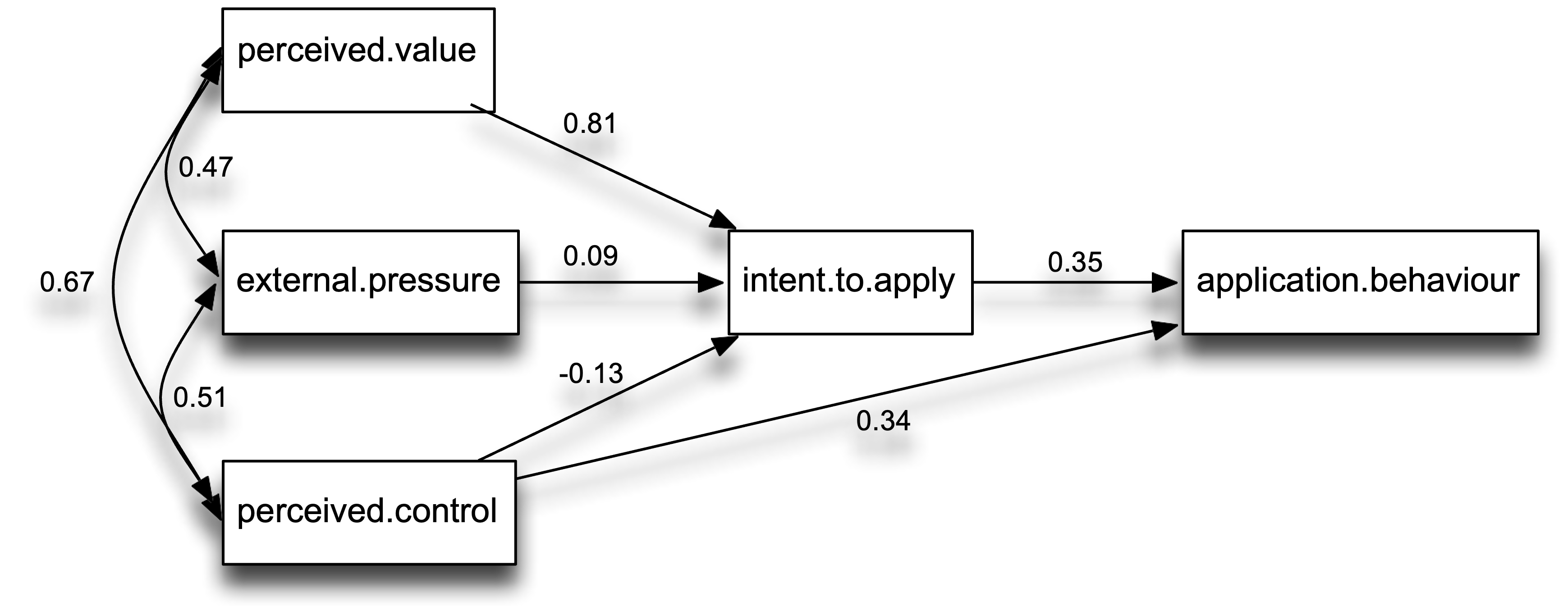
Visualize model

library(semPlot)
# Example of plotting the variables in specific locations
locations = matrix(c(0, 0, .5, 0, -.5, .5, -.5, 0, -.5, -.5), ncol=2, byrow=2)
labels = c("Intent\nTo Apply","Application\nBehaviour","Perceived\nValue","External\nPressure","Perceived\nControl")
diagram = semPaths(fit, whatLabels="std", nodeLabels = labels, layout=locations, sizeMan = 12, rotation=2)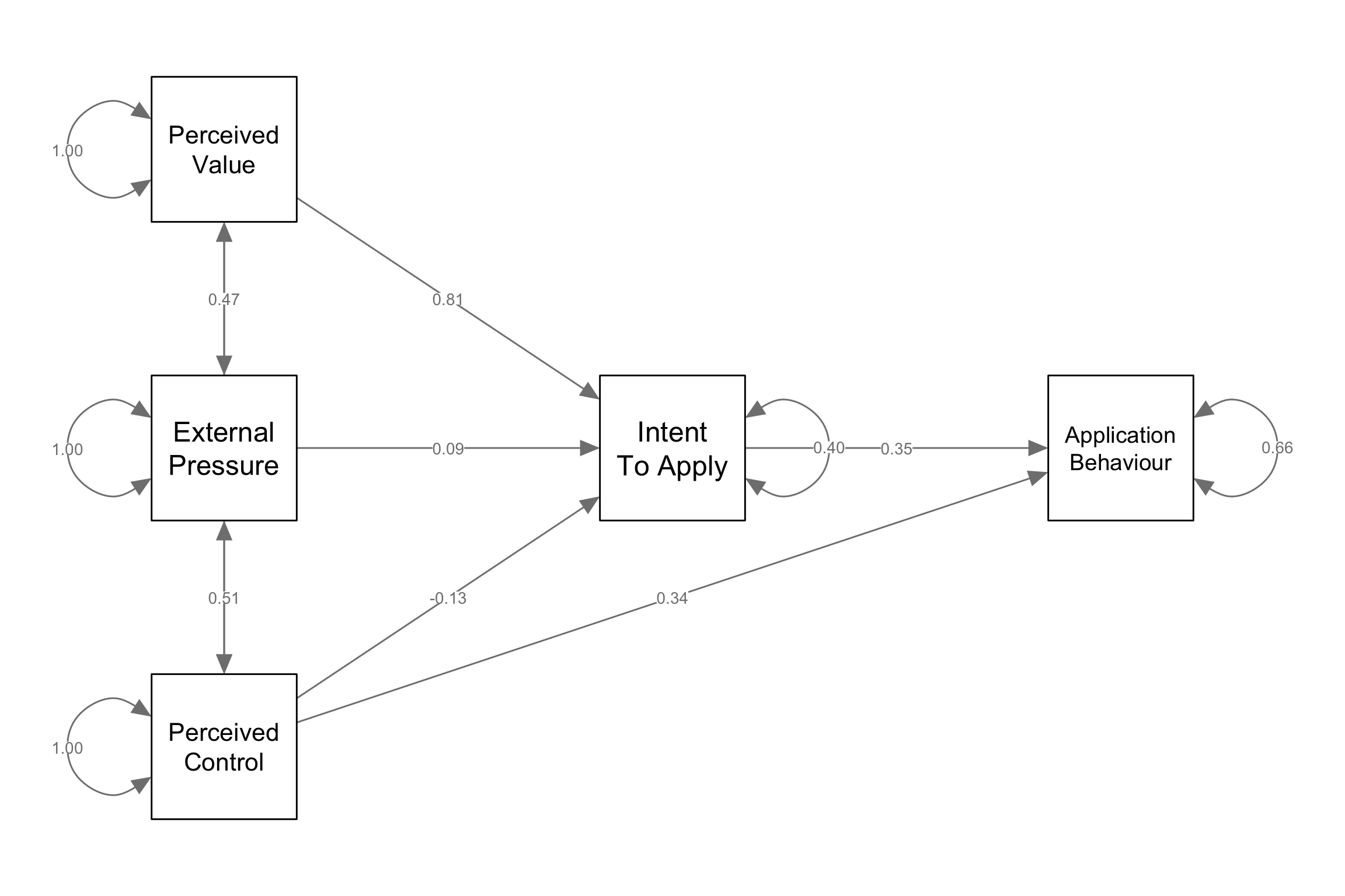

Bad fit

• What if fit incidences are not that good?

• Modification (mod) indices

  • Tell you what the chi-square change would be if you added the path suggested

  • Can make your model better

    • Potential for HARKING!
    • Be transparent

Modifications

• Modification indices (look at mi column)

modificationindices(fit)

lhs	op	rhs	mi	epc	sepc.lv	sepc.all	sepc.nox
intent.to.apply	~~	application.behaviour	0.50	-4.20	-4.20	-0.13	-0.13
application.behaviour	~~	perceived.value	0.14	4.31	4.31	0.05	0.05
application.behaviour	~~	external.pressure	0.43	11.74	11.74	0.07	0.07
application.behaviour	~~	perceived.control	0.79	-15.98	-15.98	-0.16	-0.16
intent.to.apply	~	application.behaviour	0.50	-0.02	-0.02	-0.10	-0.10
application.behaviour	~	perceived.value	0.35	0.28	0.28	0.12	0.12

•  Anything with \(\chi^2(1)\) > 3.84 is *p* < .05

Best practices

• Comparing multiple models

  • Constraining paths

    • In SEM you can explicitly test hypotheses about the size of specific paths

      • Constrain a path to certain value

      • Constrain two paths to be equal

        • Compare model fit of models with constrained and unconstrained paths

  • Assess alternative hypotheses/models

Constraining paths

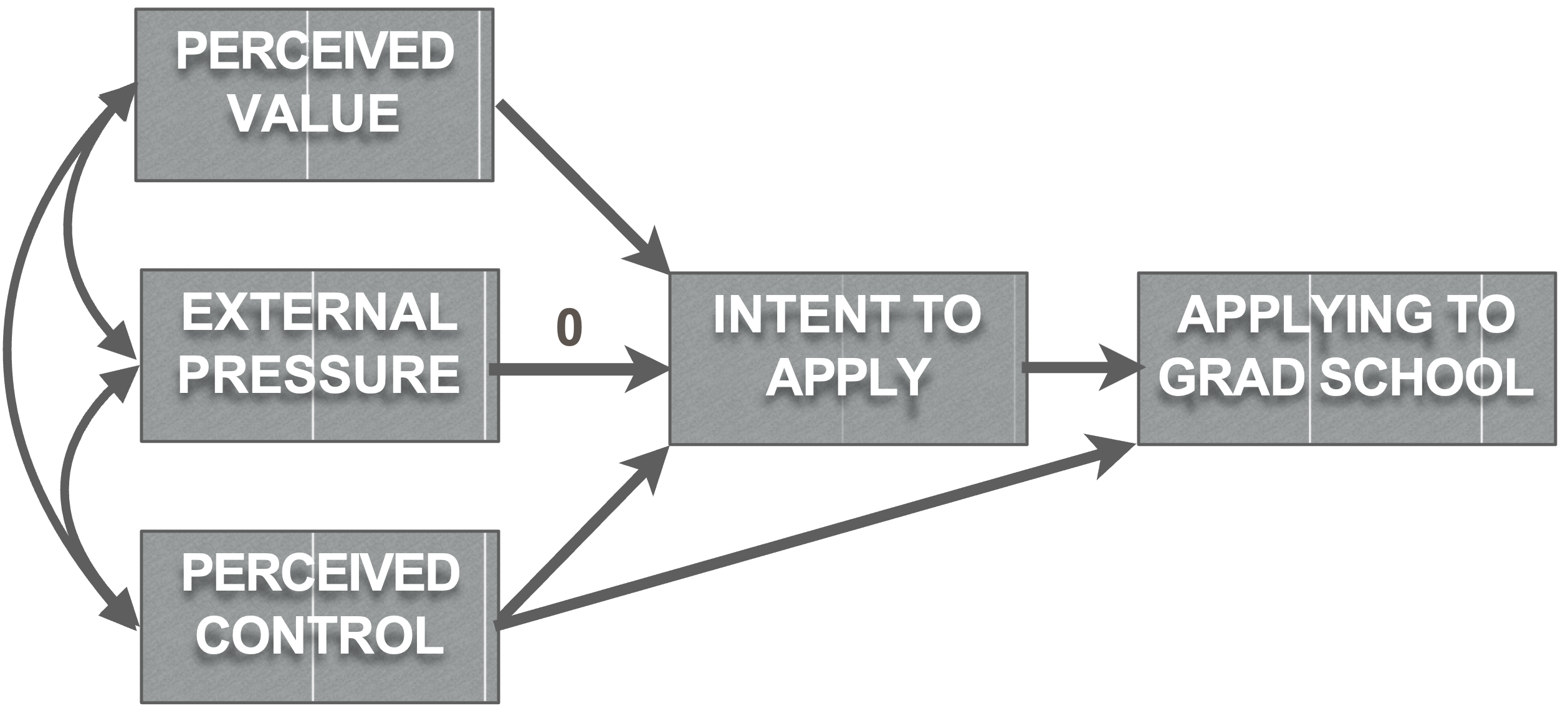
grad_model_constrained =  '
  intent.to.apply ~ a*perceived.value + 0*external.pressure + c*perceived.control
  application.behaviour ~ d*intent.to.apply + perceived.control

  perceived.control ~~ perceived.value # These are covariance paths
  perceived.control ~~ external.pressure # These are covariance paths
  external.pressure ~~ perceived.value # These are covariance paths

  value.through.intent:=a*d
  control.through.intent:=c*d
'

grad_analysis_constrained = 
 sem(grad_model_constrained, data=grad, se="bootstrap")

Nested model comparisons

• If you can create one model from another by the addition or subtraction of parameters, then it is nested

  • Model A is said to be nested within Model B, if Model B is a more complicated version of Model A

• Evaluating models

  • Ensure both fit data well

    • Report comparative fit indices
    • If one sucks, go with least crappy one
    • If both suck, don’t compare them

• Use LRT test

LRT test

• Test both model fits

performance::compare_performance(fit, grad_analysis_constrained) %>% kable()

Name	Model	Chi2	Chi2_df	p_Chi2	Baseline	Baseline_df	p_Baseline	GFI	AGFI	NFI	NNFI	CFI	RMSEA	RMSEA_CI_low	RMSEA_CI_high	p_RMSEA	RMR	SRMR	RFI	PNFI	IFI	RNI	Loglikelihood	AIC	AIC_wt	BIC	BIC_wt	BIC_adjusted
fit	lavaan	0.8615836	2	0.6499942	136.416	10	0	0.9943295	0.9574712	0.9936841	1.045027	1	0	0	0.1997409	0.6896164	3.564326	0.0190206	0.9684207	0.1987368	1.008469	1.009005	-993.7334	2013.467	0.3717899	2040.693	0.1719716	1999.805
grad_analysis_constrained	lavaan	1.8124921	3	0.6122203	136.416	10	0	0.9886592	0.9432959	0.9867135	1.031312	1	0	0	0.1794375	0.6671659	4.826403	0.0301489	0.9557116	0.2960140	1.008901	1.009394	-994.2089	2012.418	0.6282101	2037.550	0.8280284	1999.807

• \(\Delta\) \(\chi^2\) (note: Constraining a path adds 1 df (the model with more DFs is more parsimonious)

test_likelihoodratio(fit, grad_analysis_constrained) %>% knitr::kable(., digits = 3)

Model	Type	df	df_diff	Chi2	p
fit	lavaan	2	NA	0.862	NA
grad_analysis_constrained	lavaan	3	1	1.812	0.329

Non-nested model comparisons

#nonntested model
grad_model_nonnested = '
  intent.to.apply ~ a*perceived.value
  application.behaviour ~ b*intent.to.apply + c*job.opportunities
  #indirect1
  indirect:= a*b

  perceived.value ~~ job.opportunities # Covariance path between 2 exogenous variables
'

• Ensure both models fit well

  • If so, compare models with AIC or BIC (go with lowest)

  • If not, choose model that fits

  • Use compare_performance() from easystats

# compare these models
performance::compare_performance(fit, grad_model_nonnested) %>% kable()

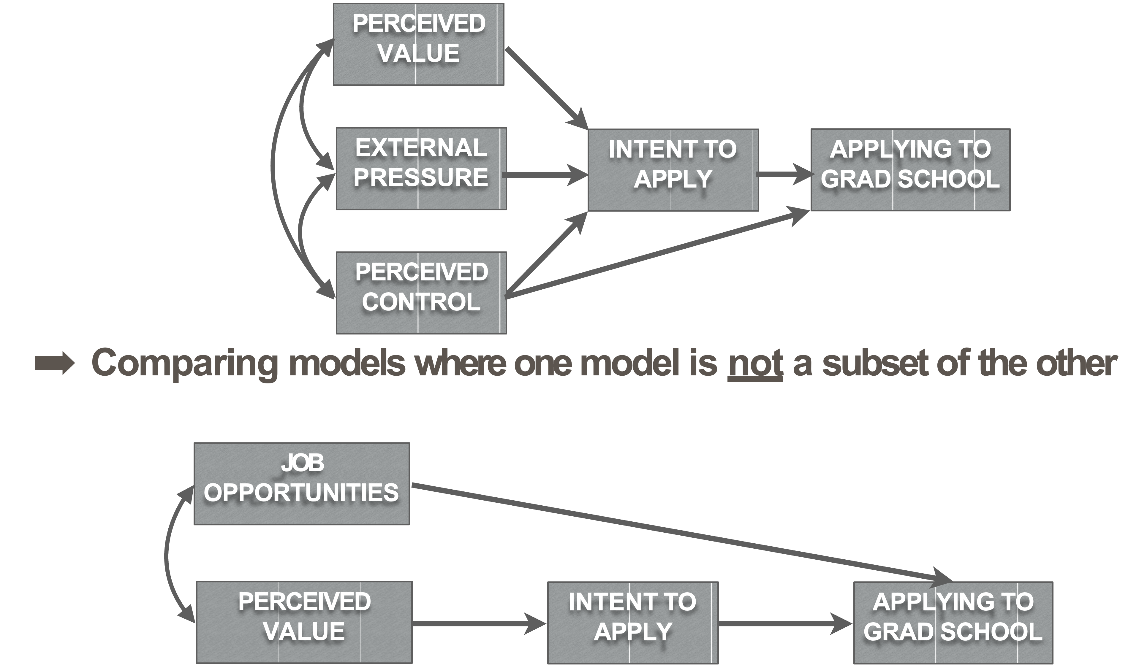
Write-up: Nested models

We wanted to see if the data fit Ajzen’s (1985) Theory of planned behavior (“Unconstrained Model,” Figure 1) better than a constrained model that posits no relationship between external pressure and intention to apply to graduate school (“Constrained Model,” Figure 2). The constrained model fit the data well, SRMR = .03, RMSEA = 0, 90% CI [0, 0.18], CFI = 1, AIC = 2000.42, BIC = 2012.98. A Likelihood Ratio test of the two models suggested that the models fit the data equally well, \(\chi^2\) (1) = 0.95, p = 0.33. Thus, we trimmed this path in the interest of parsimony. 

Write-up: Non-nested

We also compared a non-nested model that considered the strongest pathway of our originally hypothesized model in the context of job opportunities (“Opportunities Model,” Figure 3). The opportunities model had good absolute and relative goodness of fit but the relative badness of fit was poor, SRMR = .05, RMSEA =0.28, 90% CI [0.13, 0.44], CFI = 0.96, AIC = 1502.77, BIC = 1519.52. Comparing the Opportunities Model to the Hypothesized Model (Figure 1) using BIC (Kass & Raftery, 1995) reveals that the evidence strongly favors the Opportunities Model, \(BIC_{Hypothesized}\) = 2040.69, ΔBIC= 521.

Practical issues

• Sample size: for parameter estimates to be accurate, you should have large samples

• How many? Hard to say, but often hundreds are necessary

  • http://web.pdx.edu/~newsomj/semclass/ho_sample%20size.pdf
  • https://www.ncbi.nlm.nih.gov/pmc/articles/PMC4334479/

• Check out Greg Hancock’s talk https://drive.google.com/file/d/1U6UyYZCJ0sW1muKQZ-VNn9EIBtGWH_uS/view?usp=sharing

  • Provides a simple way to calculate power/sample size

Practical issues

• Sample Size: The N:q rule
  • Number of people, N
  • q number of estimated parameters
  • You want the N:q ratio to be 20:1 or greater in a perfect world, 10:1 if you can manage it, at the bare minimum 5:1.

Assumptions

• All assumptions for linear models apply to SEM
• There are robust estimators one can use
  • Sattorra-Bentler
    • sem(model, test="satorra.bentler")

SEM: Summary

• SEM is a statistical technique that combines path analysis and factor analysis to allow for statistical modeling of the relationships between observed variables and latent constructs

• It focuses heavily on model fit to evaluate how well the proposed model fits the data

• It’s a very flexible analysis that has several variations, extensions, and applications

Announcements

• Lab

  • No lab on Wednesday

    • We will incorporate SEM into factor analysis lab next week

• Next week

  • Factor analysis (Aditi and Brooke)

• Free SEM workshop

  • May 8th-10th

    • https://centerstat.org/structural-equation-modeling/

Acknowledgments

• Thanks to Elizabeth Page-Gould, Chris Groves, and Erin Buchanan for graciously providing some of the content I used here