Introduction to Exploratory and Confirmatory Factor Analysis (Using R)
Princeton University
2024-04-22
Today
Exploratory (common) factor analysis
What is it?
Why?
Variance
FA vs. PCA
Carrying out exploratory factor analysis in R
CFA
Visualization and reporting factor analysis
Packages
What is factor analysis?
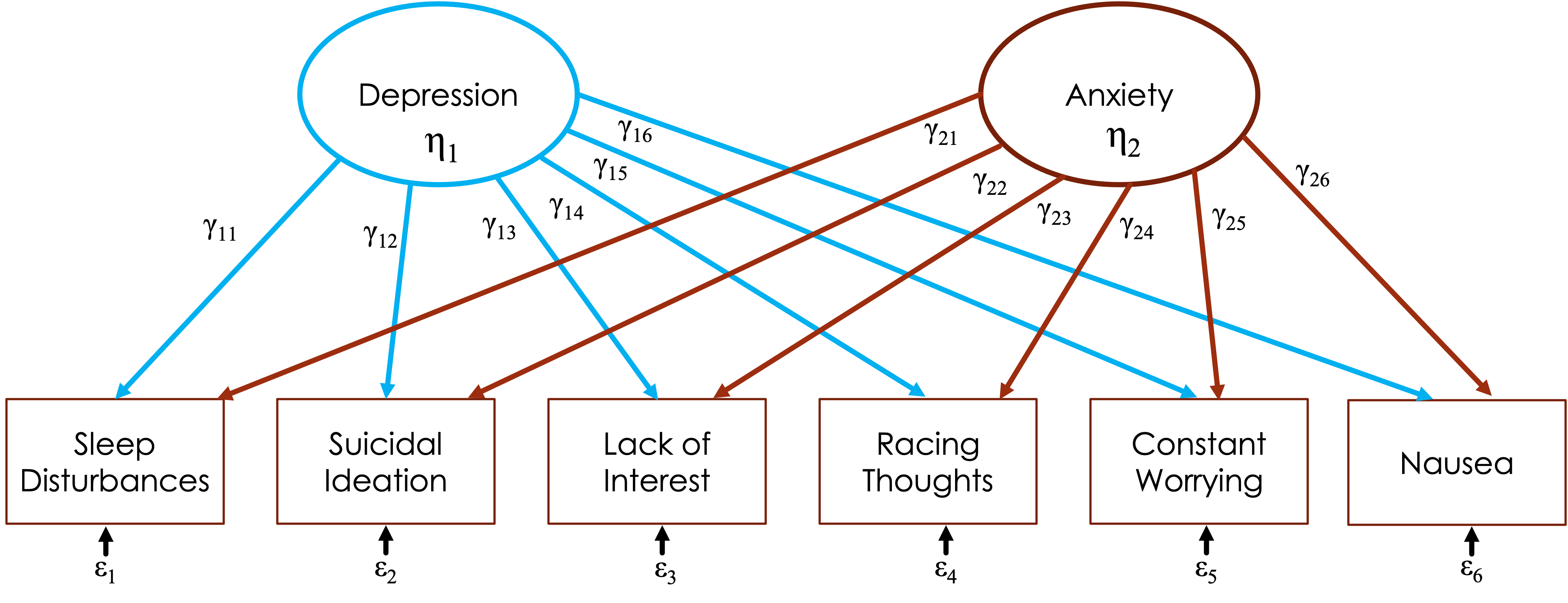
Let’s say we have 6 items in a scale:
Sleep disturbances (insomnia/hypersomnia)
Suicidal ideation
Lack of interest in normally engaging activities
Racing thoughts
Constant worrying
Nausea
- FA “looks” at the relationships between these items and finds that some of them seem to hang together
What is factor analysis?
Let’s say we have 6 items in a scale:
Sleep disturbances (insomnia/hypersomnia)
Suicidal ideation
Lack of interest in normally engaging activities
Racing thoughts
Constant worrying
Nausea
Some of these could cross-load
FA considers this and items load on all factors
Why?
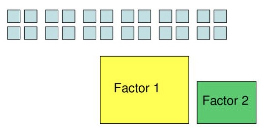
Allows you to summarize complex data with a smaller set of representative variables
- 6 variables to 2 variables
Why?
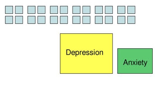
Can help identify/confirm underlying constructs
- Depression and anxiety
Partitioning variance
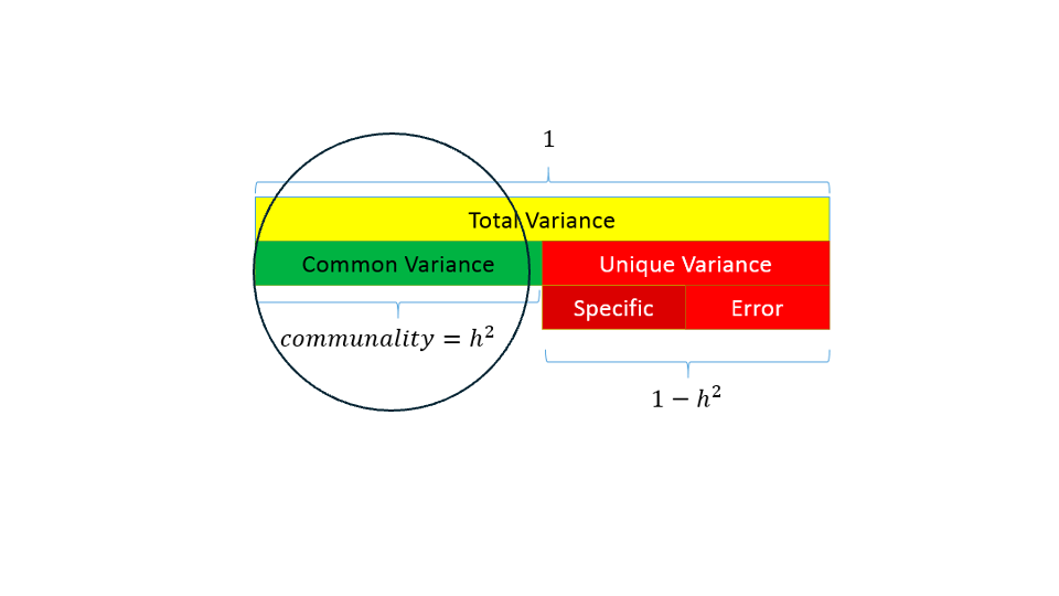
Variance common to other variables
- Communality \(h^2\): proportion of each variable’s/item’s variance that can be explained by the factors
- How much an item is related to other items in the analysis
- Communality \(h^2\): proportion of each variable’s/item’s variance that can be explained by the factors
Variance specific to that variable (unique variance)
Random measurement error
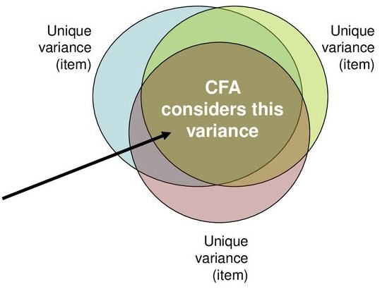
Common factor analysis
Common factor analysis
- Attempts to achieve parsimony (data reduction) by:
- Explaining the maximum amount of common variance in a correlation matrix
- Using the smallest number of explanatory constructs (factors)
- Explaining the maximum amount of common variance in a correlation matrix
- Attempts to achieve parsimony (data reduction) by:
Common factor analysis
Partitions variance that is in common with other variables. How?
Use multiple regression to calculate multiple \(R^2\)
Each item as an outcome
Use all other items as predictors
Finds the communality among all of the variables, relative to one another
Common factor analysis

Common factor analysis

Common factor analysis

PCA
- Based on total variance!

- Goal: Find fewest components that accounts for the most varaiance among variables
PCA vs. FA
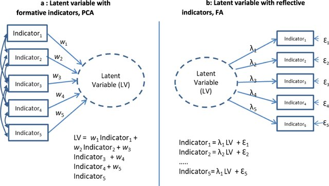
Run factor analysis if you assume or wish to test a theoretical model of latent factors causing observed variables
Run PCA If you want to simply reduce your correlated observed variables to a smaller set of important independent composite variables
Eigenvalues and Eigenvectors
Eigenvalues represent the total amount of variance that can be explained by a given factor
- Sum of squared component loadings down all items for each factor
Eigenvectors represent a weight for each eigenvalue
Eigenvector times the square root of the eigenvalue gives the factor loadings
- Correlation between item and factor
Exploratory factor analysis steps
Checking the suitability of data (should we run a factor analysis?)
Decide # of factors
Factor Extraction
Factor Rotation (make factors more interpretable)
Interpret/name
Big 5

2800 participants
25 self-report items from big 5 inventory
- The personality items are split into 5 categories
Data
Data visualization

Note
Always include correlation table in factor analysis!
Is factor analysis warranted?
Bartlett’s test
Is the Correlation matrix significantly different from an identity matrix (0s)?
1 0 0 0 1 0 0 0 1
Yes. There are correlations between the variables
No. No correlations and factor analysis is not suitable
Is factor analysis warranted?
- Kaiser-Meyer-Olkin (KMO)
\[ KMO = \frac{\Sigma(r)^2}{\Sigma(r)^2 + \Sigma(r_p)^2} \]
If variables share a common factor they will have small partial correlation (i.e., most of the variance is explained by common factor so not much left)
KMO Criterion Adequacy Interpretation 0.70-0.79 Good 0.80-0.89 Very Good 0.90-1.00 Excellent
Is factor analysis warranted?
# Is the data suitable for Factor Analysis?


  - Sphericity: Bartlett's test of sphericity suggests that there is sufficient significant correlation in the data for factor analysis (Chisq(276) = 17568.93, p < .001).
- KMO: The Kaiser, Meyer, Olkin (KMO) overall measure of sampling adequacy suggests that data seems appropriate for factor analysis (KMO = 0.85). The individual KMO scores are: A1 (0.74), A2 (0.84), A3 (0.87), A4 (0.88), A5 (0.90), C1 (0.84), C2 (0.79), C3 (0.86), C4 (0.82), C5 (0.86), E1 (0.84), E2 (0.88), E3 (0.89), E4 (0.88), E5 (0.89), N1 (0.78), N2 (0.78), N3 (0.86), N4 (0.89), N5 (0.86), O1 (0.84), O2 (0.72), O3 (0.83), O4 (0.75).- Check’s Bartlett’s
- Checks KMO
- Check MSA (should delete item MSA < .5)
Assumptions
No outliers
Large sample
- 100
Normality
No missingness
No multicollinearity
Assumptions: Outliers
82 outliers detected: cases 31, 42, 48, 149, 170, 236, 287, 325, 359,
  373, 376, 399, 400, 418, 488, 490, 581, 661, 702, 707, 727, 729, 756,
  774, 776, 779, 825, 843, 882, 883, 995, 1005, 1015, 1032, 1059, 1077,
  1082, 1116, 1121, 1136, 1160, 1248, 1282, 1314, 1315, 1318, 1321, 1365,
  1369, 1370, 1374, 1375, 1376, 1377, 1442, 1545, 1549, 1552, 1566, 1693,
  1746, 1763, 1783, 1794, 1805, 1823, 1824, 1873, 1914, 1944, 2027, 2195,
  2203, 2266, 2268, 2272, 2281, 2324, 2355, 2402, 2407, 2422.
- Based on the following method and threshold: mahalanobis (51.179).
- For variables: A1, A2, A3, A4, A5, C1, C2, C3, C4, C5, E1, E2, E3, E4,
E5, N1, N2, N3, N4, N5, O1, O2, O3, O4.Assumptions: Multicollinearity
We do not want variables that are too highly correlated
Determinant of correlation matrix
- Smaller < .00001 (close to 0) suggests a problem with multicollinearity
Fitting factor model: # of factors
Several different ways:
A priori
Eigenvalues > 1 (Kaiser criterion)
Cumulative percent variance extracted (75%)
Fitting factor model: # of factors
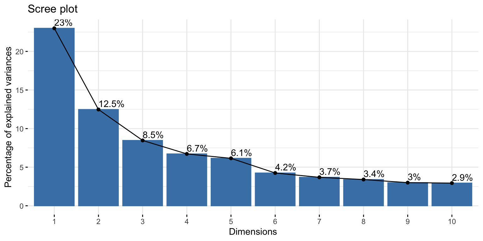
Scree plot
A plot of the Eigenvalues in order from largest to smallest
Look for the elbow (shared variability starting to level off)
- Above the elbow is how many components you want
Fitting factor model: # of factors
Parallel analysis
Run simulations pulling eigenvalues from randomly generated datasets (with same sample size and number of variables)
If eigenvalues > eigenvalues from random datasets more likely to represent meaningful patterns in the data
Method agreement procedure
Uses many methods to determine how many factor you should get
- This is the approach I would use

Extracting factor loadings
Runs another factor analysis to get the loading for each of the factors
- Principal axis factoring (PAF)
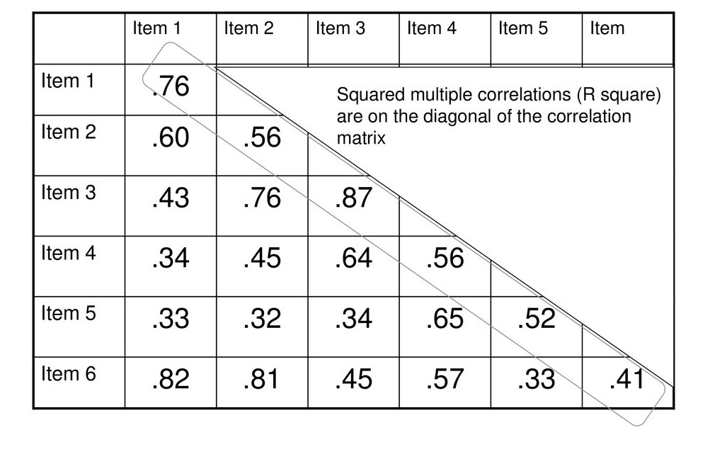
- Get initial estimates of communalities
- Squared multiple correlations (highest absolute correlation)
- Take correlation matrix and replace diagonal elements with communalities (reduced matrix)
- Principal axis factoring (PAF)
Running factor analysis
# nfactor number of factors from par analysis
# rotate rotation method
# fm is principle axis
efa <- psych::fa(data, nfactors = 5, rotate="none", fm="pa")

efa
Factor Analysis using method = pa
Call: psych::fa(r = data, nfactors = 5, rotate = "none", fm = "pa")
Standardized loadings (pattern matrix) based upon correlation matrix
PA1 PA2 PA3 PA4 PA5 h2 u2 com
A1 -0.23 0.00 0.15 -0.18 -0.33 0.22 0.78 2.9
A2 0.48 0.28 -0.17 0.28 0.25 0.47 0.53 3.2
A3 0.54 0.30 -0.24 0.24 0.22 0.54 0.46 2.9
A4 0.43 0.13 -0.05 0.32 0.06 0.30 0.70 2.1
A5 0.59 0.17 -0.26 0.14 0.13 0.49 0.51 1.8
C1 0.34 0.15 0.47 0.01 0.03 0.36 0.64 2.1
C2 0.33 0.22 0.53 0.14 0.02 0.45 0.55 2.3
C3 0.33 0.10 0.42 0.19 -0.03 0.33 0.67 2.5
C4 -0.47 0.07 -0.50 -0.13 0.07 0.49 0.51 2.2
C5 -0.51 0.12 -0.36 -0.15 0.16 0.45 0.55 2.4
E1 -0.42 -0.18 0.27 0.12 0.24 0.35 0.65 3.1
E2 -0.64 -0.05 0.21 0.12 0.30 0.56 0.44 1.8
E3 0.54 0.32 -0.16 -0.21 -0.01 0.46 0.54 2.2
E4 0.61 0.17 -0.29 0.05 -0.23 0.55 0.45 2.0
E5 0.52 0.30 0.10 -0.16 -0.19 0.43 0.57 2.2
N1 -0.45 0.64 0.05 0.00 -0.28 0.70 0.30 2.2
N2 -0.44 0.63 0.08 -0.02 -0.22 0.65 0.35 2.1
N3 -0.42 0.61 0.02 0.06 -0.02 0.56 0.44 1.8
N4 -0.54 0.40 0.04 0.02 0.23 0.51 0.49 2.2
N5 -0.35 0.42 0.00 0.25 0.05 0.36 0.64 2.7
O1 0.32 0.21 0.12 -0.43 0.18 0.37 0.63 3.0
O2 -0.17 0.07 -0.21 0.33 -0.19 0.23 0.77 3.1
O3 0.38 0.29 0.04 -0.47 0.21 0.50 0.50 3.1
O4 -0.09 0.24 0.09 -0.15 0.39 0.25 0.75 2.3
PA1 PA2 PA3 PA4 PA5
SS loadings 4.73 2.28 1.54 1.09 0.95
Proportion Var 0.20 0.10 0.06 0.05 0.04
Cumulative Var 0.20 0.29 0.36 0.40 0.44
Proportion Explained 0.45 0.22 0.15 0.10 0.09
Cumulative Proportion 0.45 0.66 0.81 0.91 1.00
Mean item complexity = 2.4
Test of the hypothesis that 5 factors are sufficient.
df null model = 276 with the objective function = 7.56 with Chi Square = 17793.19
df of the model are 166 and the objective function was 0.55
The root mean square of the residuals (RMSR) is 0.03
The df corrected root mean square of the residuals is 0.03
The harmonic n.obs is 2363 with the empirical chi square 874.77 with prob < 0.000000000000000000000000000000000000000000000000000000000000000000000000000000000000000000000001
The total n.obs was 2363 with Likelihood Chi Square = 1294.25 with prob < 0.0000000000000000000000000000000000000000000000000000000000000000000000000000000000000000000000000000000000000000000000000000000000000000000000000000000000000000000000000000069
Tucker Lewis Index of factoring reliability = 0.893
RMSEA index = 0.054 and the 90 % confidence intervals are 0.051 0.056
BIC = 4.81
Fit based upon off diagonal values = 0.99
Measures of factor score adequacy
PA1 PA2 PA3 PA4 PA5
Correlation of (regression) scores with factors 0.95 0.92 0.86 0.81 0.80
Multiple R square of scores with factors 0.90 0.84 0.73 0.65 0.64
Minimum correlation of possible factor scores 0.81 0.68 0.47 0.30 0.28Factor loadings
Pattern matrix
- Correlation between item and factor
| Variable | PA1 | PA2 | PA3 | PA4 | PA5 | Complexity | Uniqueness |
|---|---|---|---|---|---|---|---|
| A1 | -0.2319882 | 0.0023261 | 0.1455464 | -0.1847440 | -0.3270490 | 2.927691 | 0.7839009 |
| A2 | 0.4784454 | 0.2801784 | -0.1668768 | 0.2782523 | 0.2467249 | 3.248297 | 0.5264446 |
| A3 | 0.5409350 | 0.2966276 | -0.2384365 | 0.2385150 | 0.2246832 | 2.899315 | 0.4551774 |
| A4 | 0.4257303 | 0.1277657 | -0.0539147 | 0.3165498 | 0.0622511 | 2.148040 | 0.6954438 |
| A5 | 0.5926797 | 0.1746998 | -0.2628775 | 0.1443625 | 0.1267702 | 1.833381 | 0.5121950 |
| C1 | 0.3431614 | 0.1505685 | 0.4722258 | 0.0068654 | 0.0328632 | 2.072997 | 0.6354450 |
| C2 | 0.3305886 | 0.2186915 | 0.5262570 | 0.1380051 | 0.0155291 | 2.251248 | 0.5466523 |
| C3 | 0.3274511 | 0.0953709 | 0.4193421 | 0.1943316 | -0.0267108 | 2.488719 | 0.6693541 |
| C4 | -0.4660709 | 0.0747389 | -0.4986585 | -0.1259735 | 0.0657961 | 2.211288 | 0.5083333 |
| C5 | -0.5075724 | 0.1156175 | -0.3562129 | -0.1512068 | 0.1597062 | 2.375683 | 0.5537457 |
| E1 | -0.4159372 | -0.1764771 | 0.2671205 | 0.1236466 | 0.2415778 | 3.075999 | 0.6508504 |
| E2 | -0.6413885 | -0.0505221 | 0.2114952 | 0.1217465 | 0.3001144 | 1.768602 | 0.4364472 |
| E3 | 0.5350316 | 0.3191105 | -0.1590188 | -0.2145295 | -0.0129357 | 2.221514 | 0.5404324 |
| E4 | 0.6138901 | 0.1740996 | -0.2910524 | 0.0519395 | -0.2266817 | 1.951200 | 0.4540345 |
| E5 | 0.5246185 | 0.2951107 | 0.1007719 | -0.1623253 | -0.1892551 | 2.211699 | 0.5653632 |
| N1 | -0.4498689 | 0.6444939 | 0.0478371 | 0.0002313 | -0.2756512 | 2.209375 | 0.3039736 |
| N2 | -0.4445789 | 0.6281875 | 0.0824668 | -0.0241956 | -0.2212982 | 2.133086 | 0.3513709 |
| N3 | -0.4211979 | 0.6138197 | 0.0213682 | 0.0626791 | -0.0233814 | 1.802314 | 0.4408857 |
| N4 | -0.5441809 | 0.4048843 | 0.0375723 | 0.0233649 | 0.2257279 | 2.245888 | 0.4870251 |
| N5 | -0.3533213 | 0.4162629 | -0.0003564 | 0.2475460 | 0.0520310 | 2.655716 | 0.6379029 |
| O1 | 0.3197803 | 0.2069097 | 0.1156597 | -0.4251826 | 0.1781743 | 2.981538 | 0.6290254 |
| O2 | -0.1724746 | 0.0738966 | -0.2117031 | 0.3323978 | -0.1876405 | 3.112332 | 0.7742764 |
| O3 | 0.3826257 | 0.2941170 | 0.0380693 | -0.4687009 | 0.2121736 | 3.144443 | 0.5009454 |
| O4 | -0.0926238 | 0.2441655 | 0.0877732 | -0.1481268 | 0.3911883 | 2.281420 | 0.7491301 |
Naming: PA1-PA2…
- Reflects fitting method
| Variable | PA1 | PA2 | PA3 | PA4 | PA5 | Complexity | Uniqueness |
|---|---|---|---|---|---|---|---|
| A1 | -0.2319882 | 0.0023261 | 0.1455464 | -0.1847440 | -0.3270490 | 2.927691 | 0.7839009 |
| A2 | 0.4784454 | 0.2801784 | -0.1668768 | 0.2782523 | 0.2467249 | 3.248297 | 0.5264446 |
| A3 | 0.5409350 | 0.2966276 | -0.2384365 | 0.2385150 | 0.2246832 | 2.899315 | 0.4551774 |
| A4 | 0.4257303 | 0.1277657 | -0.0539147 | 0.3165498 | 0.0622511 | 2.148040 | 0.6954438 |
| A5 | 0.5926797 | 0.1746998 | -0.2628775 | 0.1443625 | 0.1267702 | 1.833381 | 0.5121950 |
| C1 | 0.3431614 | 0.1505685 | 0.4722258 | 0.0068654 | 0.0328632 | 2.072997 | 0.6354450 |
| C2 | 0.3305886 | 0.2186915 | 0.5262570 | 0.1380051 | 0.0155291 | 2.251248 | 0.5466523 |
| C3 | 0.3274511 | 0.0953709 | 0.4193421 | 0.1943316 | -0.0267108 | 2.488719 | 0.6693541 |
| C4 | -0.4660709 | 0.0747389 | -0.4986585 | -0.1259735 | 0.0657961 | 2.211288 | 0.5083333 |
| C5 | -0.5075724 | 0.1156175 | -0.3562129 | -0.1512068 | 0.1597062 | 2.375683 | 0.5537457 |
| E1 | -0.4159372 | -0.1764771 | 0.2671205 | 0.1236466 | 0.2415778 | 3.075999 | 0.6508504 |
| E2 | -0.6413885 | -0.0505221 | 0.2114952 | 0.1217465 | 0.3001144 | 1.768602 | 0.4364472 |
| E3 | 0.5350316 | 0.3191105 | -0.1590188 | -0.2145295 | -0.0129357 | 2.221514 | 0.5404324 |
| E4 | 0.6138901 | 0.1740996 | -0.2910524 | 0.0519395 | -0.2266817 | 1.951200 | 0.4540345 |
| E5 | 0.5246185 | 0.2951107 | 0.1007719 | -0.1623253 | -0.1892551 | 2.211699 | 0.5653632 |
| N1 | -0.4498689 | 0.6444939 | 0.0478371 | 0.0002313 | -0.2756512 | 2.209375 | 0.3039736 |
| N2 | -0.4445789 | 0.6281875 | 0.0824668 | -0.0241956 | -0.2212982 | 2.133086 | 0.3513709 |
| N3 | -0.4211979 | 0.6138197 | 0.0213682 | 0.0626791 | -0.0233814 | 1.802314 | 0.4408857 |
| N4 | -0.5441809 | 0.4048843 | 0.0375723 | 0.0233649 | 0.2257279 | 2.245888 | 0.4870251 |
| N5 | -0.3533213 | 0.4162629 | -0.0003564 | 0.2475460 | 0.0520310 | 2.655716 | 0.6379029 |
| O1 | 0.3197803 | 0.2069097 | 0.1156597 | -0.4251826 | 0.1781743 | 2.981538 | 0.6290254 |
| O2 | -0.1724746 | 0.0738966 | -0.2117031 | 0.3323978 | -0.1876405 | 3.112332 | 0.7742764 |
| O3 | 0.3826257 | 0.2941170 | 0.0380693 | -0.4687009 | 0.2121736 | 3.144443 | 0.5009454 |
| O4 | -0.0926238 | 0.2441655 | 0.0877732 | -0.1481268 | 0.3911883 | 2.281420 | 0.7491301 |
Complexity
- Number of factors an item loads on (ideally 1!)
| Variable | PA1 | PA2 | PA3 | PA4 | PA5 | Complexity | Uniqueness |
|---|---|---|---|---|---|---|---|
| A1 | -0.2319882 | 0.0023261 | 0.1455464 | -0.1847440 | -0.3270490 | 2.927691 | 0.7839009 |
| A2 | 0.4784454 | 0.2801784 | -0.1668768 | 0.2782523 | 0.2467249 | 3.248297 | 0.5264446 |
| A3 | 0.5409350 | 0.2966276 | -0.2384365 | 0.2385150 | 0.2246832 | 2.899315 | 0.4551774 |
| A4 | 0.4257303 | 0.1277657 | -0.0539147 | 0.3165498 | 0.0622511 | 2.148040 | 0.6954438 |
| A5 | 0.5926797 | 0.1746998 | -0.2628775 | 0.1443625 | 0.1267702 | 1.833381 | 0.5121950 |
| C1 | 0.3431614 | 0.1505685 | 0.4722258 | 0.0068654 | 0.0328632 | 2.072997 | 0.6354450 |
| C2 | 0.3305886 | 0.2186915 | 0.5262570 | 0.1380051 | 0.0155291 | 2.251248 | 0.5466523 |
| C3 | 0.3274511 | 0.0953709 | 0.4193421 | 0.1943316 | -0.0267108 | 2.488719 | 0.6693541 |
| C4 | -0.4660709 | 0.0747389 | -0.4986585 | -0.1259735 | 0.0657961 | 2.211288 | 0.5083333 |
| C5 | -0.5075724 | 0.1156175 | -0.3562129 | -0.1512068 | 0.1597062 | 2.375683 | 0.5537457 |
| E1 | -0.4159372 | -0.1764771 | 0.2671205 | 0.1236466 | 0.2415778 | 3.075999 | 0.6508504 |
| E2 | -0.6413885 | -0.0505221 | 0.2114952 | 0.1217465 | 0.3001144 | 1.768602 | 0.4364472 |
| E3 | 0.5350316 | 0.3191105 | -0.1590188 | -0.2145295 | -0.0129357 | 2.221514 | 0.5404324 |
| E4 | 0.6138901 | 0.1740996 | -0.2910524 | 0.0519395 | -0.2266817 | 1.951200 | 0.4540345 |
| E5 | 0.5246185 | 0.2951107 | 0.1007719 | -0.1623253 | -0.1892551 | 2.211699 | 0.5653632 |
| N1 | -0.4498689 | 0.6444939 | 0.0478371 | 0.0002313 | -0.2756512 | 2.209375 | 0.3039736 |
| N2 | -0.4445789 | 0.6281875 | 0.0824668 | -0.0241956 | -0.2212982 | 2.133086 | 0.3513709 |
| N3 | -0.4211979 | 0.6138197 | 0.0213682 | 0.0626791 | -0.0233814 | 1.802314 | 0.4408857 |
| N4 | -0.5441809 | 0.4048843 | 0.0375723 | 0.0233649 | 0.2257279 | 2.245888 | 0.4870251 |
| N5 | -0.3533213 | 0.4162629 | -0.0003564 | 0.2475460 | 0.0520310 | 2.655716 | 0.6379029 |
| O1 | 0.3197803 | 0.2069097 | 0.1156597 | -0.4251826 | 0.1781743 | 2.981538 | 0.6290254 |
| O2 | -0.1724746 | 0.0738966 | -0.2117031 | 0.3323978 | -0.1876405 | 3.112332 | 0.7742764 |
| O3 | 0.3826257 | 0.2941170 | 0.0380693 | -0.4687009 | 0.2121736 | 3.144443 | 0.5009454 |
| O4 | -0.0926238 | 0.2441655 | 0.0877732 | -0.1481268 | 0.3911883 | 2.281420 | 0.7491301 |
- 1-communality
\[ u^2_i = \varepsilon_i = 1 - \sum_{j=1}^{m}\lambda_{ij}^2 \]
| Variable | PA1 | PA2 | PA3 | PA4 | PA5 | Complexity | Uniqueness |
|---|---|---|---|---|---|---|---|
| A1 | -0.2319882 | 0.0023261 | 0.1455464 | -0.1847440 | -0.3270490 | 2.927691 | 0.7839009 |
| A2 | 0.4784454 | 0.2801784 | -0.1668768 | 0.2782523 | 0.2467249 | 3.248297 | 0.5264446 |
| A3 | 0.5409350 | 0.2966276 | -0.2384365 | 0.2385150 | 0.2246832 | 2.899315 | 0.4551774 |
| A4 | 0.4257303 | 0.1277657 | -0.0539147 | 0.3165498 | 0.0622511 | 2.148040 | 0.6954438 |
| A5 | 0.5926797 | 0.1746998 | -0.2628775 | 0.1443625 | 0.1267702 | 1.833381 | 0.5121950 |
| C1 | 0.3431614 | 0.1505685 | 0.4722258 | 0.0068654 | 0.0328632 | 2.072997 | 0.6354450 |
| C2 | 0.3305886 | 0.2186915 | 0.5262570 | 0.1380051 | 0.0155291 | 2.251248 | 0.5466523 |
| C3 | 0.3274511 | 0.0953709 | 0.4193421 | 0.1943316 | -0.0267108 | 2.488719 | 0.6693541 |
| C4 | -0.4660709 | 0.0747389 | -0.4986585 | -0.1259735 | 0.0657961 | 2.211288 | 0.5083333 |
| C5 | -0.5075724 | 0.1156175 | -0.3562129 | -0.1512068 | 0.1597062 | 2.375683 | 0.5537457 |
| E1 | -0.4159372 | -0.1764771 | 0.2671205 | 0.1236466 | 0.2415778 | 3.075999 | 0.6508504 |
| E2 | -0.6413885 | -0.0505221 | 0.2114952 | 0.1217465 | 0.3001144 | 1.768602 | 0.4364472 |
| E3 | 0.5350316 | 0.3191105 | -0.1590188 | -0.2145295 | -0.0129357 | 2.221514 | 0.5404324 |
| E4 | 0.6138901 | 0.1740996 | -0.2910524 | 0.0519395 | -0.2266817 | 1.951200 | 0.4540345 |
| E5 | 0.5246185 | 0.2951107 | 0.1007719 | -0.1623253 | -0.1892551 | 2.211699 | 0.5653632 |
| N1 | -0.4498689 | 0.6444939 | 0.0478371 | 0.0002313 | -0.2756512 | 2.209375 | 0.3039736 |
| N2 | -0.4445789 | 0.6281875 | 0.0824668 | -0.0241956 | -0.2212982 | 2.133086 | 0.3513709 |
| N3 | -0.4211979 | 0.6138197 | 0.0213682 | 0.0626791 | -0.0233814 | 1.802314 | 0.4408857 |
| N4 | -0.5441809 | 0.4048843 | 0.0375723 | 0.0233649 | 0.2257279 | 2.245888 | 0.4870251 |
| N5 | -0.3533213 | 0.4162629 | -0.0003564 | 0.2475460 | 0.0520310 | 2.655716 | 0.6379029 |
| O1 | 0.3197803 | 0.2069097 | 0.1156597 | -0.4251826 | 0.1781743 | 2.981538 | 0.6290254 |
| O2 | -0.1724746 | 0.0738966 | -0.2117031 | 0.3323978 | -0.1876405 | 3.112332 | 0.7742764 |
| O3 | 0.3826257 | 0.2941170 | 0.0380693 | -0.4687009 | 0.2121736 | 3.144443 | 0.5009454 |
| O4 | -0.0926238 | 0.2441655 | 0.0877732 | -0.1481268 | 0.3911883 | 2.281420 | 0.7491301 |
Variance accounted for
| PA1 | PA2 | PA3 | PA4 | PA5 | |
|---|---|---|---|---|---|
| SS loadings | 4.7251040 | 2.2831789 | 1.5437776 | 1.0894890 | 0.9500947 |
| Proportion Var | 0.1968793 | 0.0951325 | 0.0643241 | 0.0453954 | 0.0395873 |
| Cumulative Var | 0.1968793 | 0.2920118 | 0.3563359 | 0.4017312 | 0.4413185 |
| Proportion Explained | 0.4461162 | 0.2155642 | 0.1457543 | 0.1028631 | 0.0897023 |
| Cumulative Proportion | 0.4461162 | 0.6616804 | 0.8074346 | 0.9102977 | 1.0000000 |
Path diagram

Rotation
Make more interpretable (understandable) without actually changing the relationships among the variables
Makes high loadings higher and low/medium loadings lower
- Simple structure
- Each row contains at least one zero loading
- for each column, there are at least as many zeros as there are columns (i.e., number of factors kept)
- for any pair of factors, there are some variables with zero loadings on one factor and large loadings on the other factor
- for any pair of factors, there is a sizable proportion of zero loadings
- for any pair of factors, there is only a small number of large loadings
Rotation
Different types of rotation:
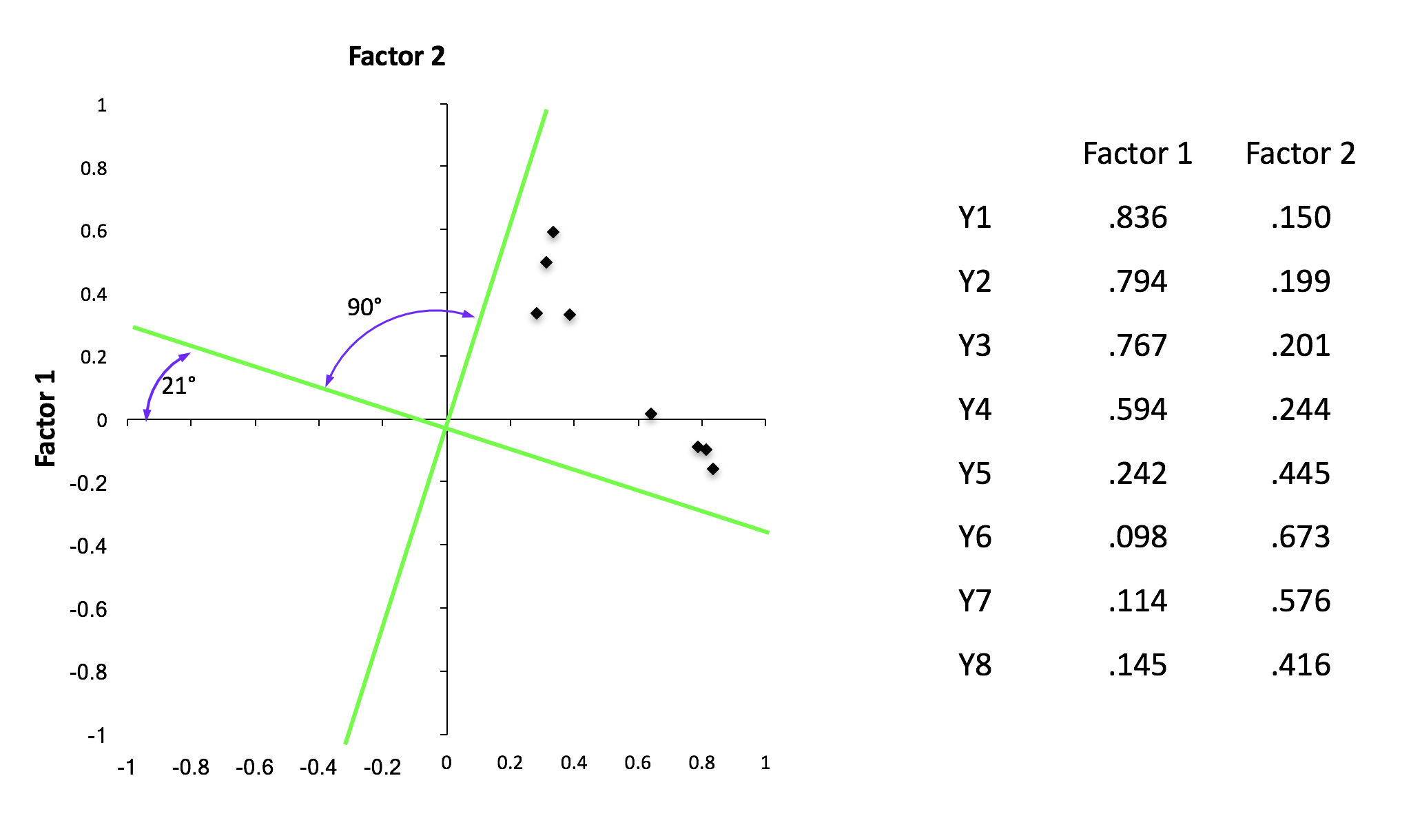
Orthogonal rotation (e.g., Varimax)
This method of rotation prevents the factors from being correlated with each other
- Rotates the axes at 90 degrees
Useful if you have factors that should theoretically be unrelated
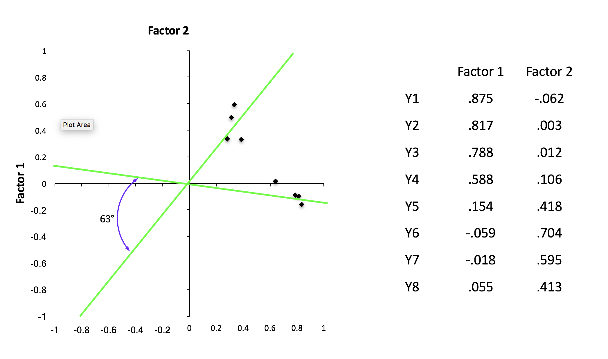
Oblique rotation (e.g., Direct Oblimin)
- Allows factors to correlate (more common)
- Good idea to always use this
Rotation

Rotation
- Orthogonal
- Oblique
Rotation
- Set
rotationargument inpsych::fa
Rotation
- After rotation

Rotation
For interpretable factor solution the convention is to eliminate small correlations (\(r\) < .32)
- Only explains 10% of the variance
Can set
thresholdargument to “max” if < .32 does not produce interpretable factors
Naming factors
PA1, PA2, etc probably not good factor names
Give factors intuitive names/labels
Highly subjective!
Use the highest loaded items to name factors
Naming factors
- Setting threshold to max works pretty well
| Variable | PA2 | PA1 | PA3 | PA5 | PA4 | Complexity | Uniqueness |
|---|---|---|---|---|---|---|---|
| N1 | 0.84 | 1.06 | 0.30 | ||||
| N2 | 0.81 | 1.04 | 0.35 | ||||
| N3 | 0.71 | 1.11 | 0.44 | ||||
| N5 | 0.50 | 2.01 | 0.64 | ||||
| N4 | 0.46 | 2.33 | 0.49 | ||||
| E2 | 0.65 | 1.12 | 0.44 | ||||
| E4 | -0.58 | 1.53 | 0.45 | ||||
| E1 | 0.54 | 1.26 | 0.65 | ||||
| E5 | -0.41 | 2.89 | 0.57 | ||||
| O4 | 0.38 | 2.40 | 0.75 | ||||
| E3 | -0.37 | 2.71 | 0.54 | ||||
| C4 | -0.67 | 1.09 | 0.51 | ||||
| C2 | 0.67 | 1.19 | 0.55 | ||||
| C3 | 0.58 | 1.08 | 0.67 | ||||
| C5 | -0.57 | 1.41 | 0.55 | ||||
| C1 | 0.57 | 1.22 | 0.64 | ||||
| A3 | 0.68 | 1.05 | 0.46 | ||||
| A2 | 0.66 | 1.03 | 0.53 | ||||
| A5 | 0.55 | 1.45 | 0.51 | ||||
| A4 | 0.46 | 1.66 | 0.70 | ||||
| A1 | -0.44 | 1.85 | 0.78 | ||||
| O3 | 0.67 | 1.03 | 0.50 | ||||
| O1 | 0.59 | 1.04 | 0.63 | ||||
| O2 | -0.42 | 2.26 | 0.77 |
The 5 latent factors (oblimin rotation) accounted for 44.13% of the total variance of the original data (PA2 = 10.90%, PA1 = 9.06%, PA3 = 9.00%, PA5 = 8.82%, PA4 = 6.36%).
What makes a good factor?
Makes sense
- Loadings on the same factor do not appear to measure completely different things
Easy to interpret
Simple structure
- Contains either high or low loadings with few moderately sized loadings
- Lacks cross-loadings
- You don’t have items that load equally onto more than 1 factor
- Keep items > .32 (or max loading)
- Throw out items with \(h^2\) < .5
- You don’t have items that load equally onto more than 1 factor
3 or more indicators per latent factor
Factor scores
Estimated scores for each participant on each underlying factor (standing on factor)
Standardize the factor loadings by dividing each loading by the square root of the sum of squares of the factor loading for that factor
Multiply scores on each item by the corresponding standardized factor loading and then summing across all items
Can use them in multiple regression!
Factor scores
Geller, J., Thye, M., & Mirman, D. (2019). Estimating effects of graded white matter damage and binary tract disconnection on post-stroke language impairment. NeuroImage, 189. https://doi.org/10.1016/j.neuroimage.2019.01.020

Plotting factor analysis
# correlated rotation
efa_obs <- psych::fa(data, nfactors = 5, rotate="oblimin", fm="pa") %>%
   model_parameters()

efa_plot <- as.data.frame(efa_obs) %>%
  pivot_longer(PA2:PA4) %>%
  dplyr::select(-Complexity, -Uniqueness) %>% rename("Loadings" = value, "Personality" = name)


#For each test, plot the loading as length and fill color of a bar
# note that the length will be the absolute value of the loading but the
# fill color will be the signed value, more on this below
efa_fact_plot <- ggplot(efa_plot, aes(Variable, abs(Loadings), fill=Loadings)) +
  facet_wrap(~ Personality, nrow=1) + #place the factors in separate facets
  geom_bar(stat="identity") + #make the bars
  coord_flip() + #flip the axes so the test names can be horizontal
  #define the fill color gradient: blue=positive, red=negative
 scale_fill_gradient2(name = "Loading",
                      high = "blue", mid = "white", low = "red",
                     midpoint=0, guide=F) +
  ylab("Loading Strength") + #improve y-axis label
  theme_bw(base_size=22)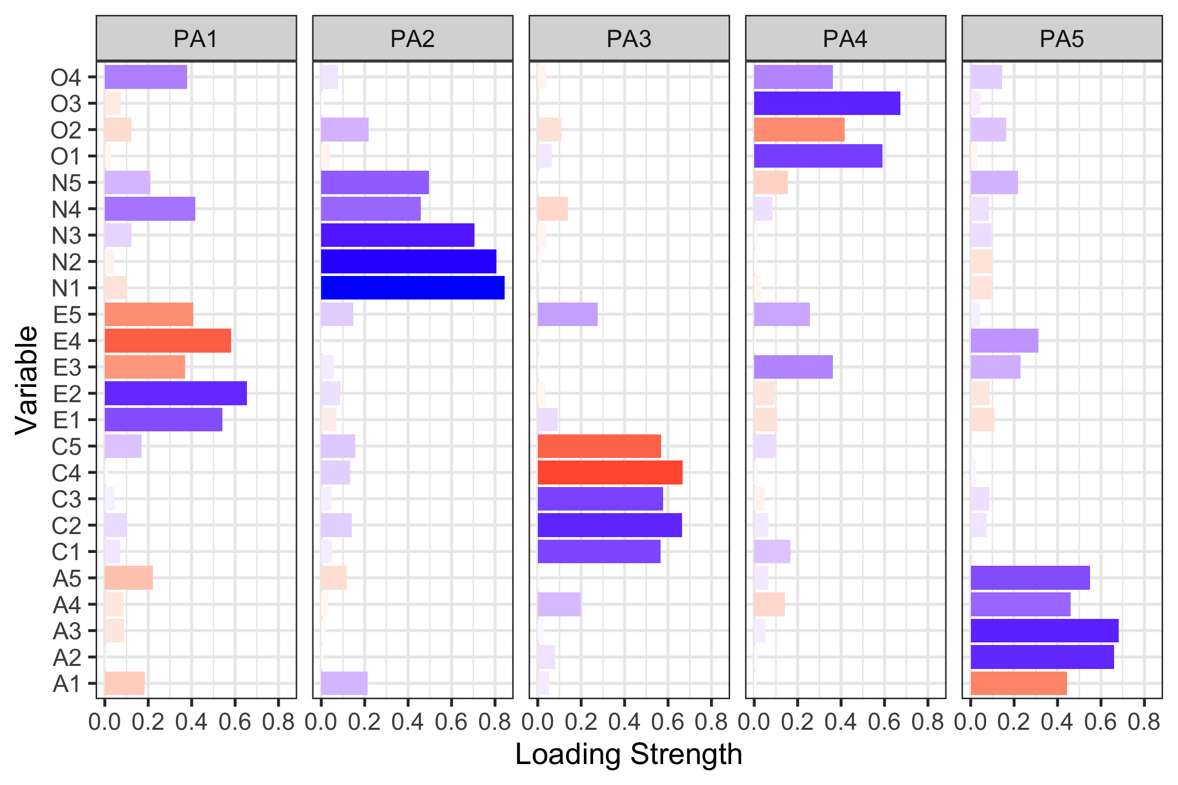
Table FA
FA table
| Factor analysis results | ||||||||
|---|---|---|---|---|---|---|---|---|
| Factor_1 | Factor_2 | Factor_3 | Factor_4 | Factor_5 | Communality | Uniqueness | Complexity | |
| N1 | 0.844 | -0.101 | 0.001 | -0.095 | -0.032 | 0.70 | 0.30 | 1.06 |
| N2 | 0.806 | -0.043 | 0.017 | -0.099 | 0.014 | 0.65 | 0.35 | 1.04 |
| N3 | 0.706 | 0.123 | -0.039 | 0.096 | 0.019 | 0.56 | 0.44 | 1.11 |
| N5 | 0.495 | 0.210 | -0.007 | 0.217 | -0.155 | 0.36 | 0.64 | 2.01 |
| N4 | 0.458 | 0.416 | -0.140 | 0.082 | 0.085 | 0.51 | 0.49 | 2.33 |
| E2 | 0.090 | 0.654 | -0.033 | -0.089 | -0.095 | 0.56 | 0.44 | 1.12 |
| E4 | 0.009 | -0.582 | 0.005 | 0.311 | -0.008 | 0.55 | 0.45 | 1.53 |
| E1 | -0.069 | 0.542 | 0.093 | -0.110 | -0.106 | 0.35 | 0.65 | 1.26 |
| E5 | 0.148 | -0.407 | 0.276 | 0.042 | 0.257 | 0.43 | 0.57 | 2.89 |
| O4 | 0.076 | 0.379 | -0.041 | 0.144 | 0.363 | 0.25 | 0.75 | 2.40 |
| E3 | 0.059 | -0.369 | -0.007 | 0.229 | 0.363 | 0.46 | 0.54 | 2.71 |
| C4 | 0.134 | 0.016 | -0.667 | 0.028 | 0.017 | 0.49 | 0.51 | 1.09 |
| C2 | 0.141 | 0.103 | 0.665 | 0.074 | 0.065 | 0.45 | 0.55 | 1.19 |
| C3 | 0.047 | 0.044 | 0.578 | 0.085 | -0.050 | 0.33 | 0.67 | 1.08 |
| C5 | 0.158 | 0.168 | -0.568 | 0.005 | 0.099 | 0.45 | 0.55 | 1.41 |
| C1 | 0.049 | 0.070 | 0.567 | 0.002 | 0.168 | 0.36 | 0.64 | 1.22 |
| A3 | -0.020 | -0.090 | 0.026 | 0.681 | 0.051 | 0.54 | 0.46 | 1.05 |
| A2 | -0.010 | -0.005 | 0.080 | 0.661 | 0.016 | 0.47 | 0.53 | 1.03 |
| A5 | -0.117 | -0.220 | -0.005 | 0.549 | 0.066 | 0.49 | 0.51 | 1.45 |
| A4 | -0.032 | -0.085 | 0.197 | 0.459 | -0.141 | 0.30 | 0.70 | 1.66 |
| A1 | 0.214 | -0.183 | 0.053 | -0.444 | -0.011 | 0.22 | 0.78 | 1.85 |
| O3 | -0.012 | -0.072 | 0.002 | 0.045 | 0.673 | 0.50 | 0.50 | 1.03 |
| O1 | -0.039 | -0.029 | 0.065 | -0.033 | 0.591 | 0.37 | 0.63 | 1.04 |
| O2 | 0.219 | -0.123 | -0.108 | 0.164 | -0.417 | 0.23 | 0.77 | 2.26 |
Confirmatory factor analysis (CFA)
EFA: tells you how many factors to retain
CFA: you already know how many factors to retain, so you test how close your data fits with expectations
Caution
- Do not do a confirmatory analysis with the same data you performed your exploratory analysis!
- Machine learning approach
Partition data training and test data
CFA in Lavaan
Let’s compare the big6 to the big5
structure_big5 <- psych::fa(training, nfactors = 5, rotate = "oblimin") %>%
  efa_to_cfa()

# Investigate how the models look
structure_big5
# Latent variables
MR2 =~ N1 + N2 + N3 + N4 + N5
MR3 =~ C1 + C2 + C3 + C4 + C5
MR1 =~ E1 + E2 + E3 + E4 + E5 + .row_id
MR5 =~ A1 + A2 + A3 + A4 + A5
MR4 =~ O1 + O2 + O3 + O4CFA in Lavaan
Fit and compare models
| Name | Model | Chi2 | Chi2_df | p (Chi2) | Baseline(300) | p (Baseline) | GFI | AGFI | NFI | NNFI | CFI | RMSEA | RMSEA CI | p (RMSEA) | RMR | SRMR | RFI | PNFI | IFI | RNI | Loglikelihood | AIC (weights) | BIC (weights) | BIC_adjusted |
|---|---|---|---|---|---|---|---|---|---|---|---|---|---|---|---|---|---|---|---|---|---|---|---|---|
| big5 | lavaan | 1434.67 | 265.00 | < .001 | 5666.19 | < .001 | 0.84 | 0.81 | 0.75 | 0.75 | 0.78 | 0.08 | [0.07, 0.08] | < .001 | 11.12 | 0.08 | 0.71 | 0.66 | 0.78 | 0.78 | -33138.25 | 66396.5 (>.999) | 66670.3 (>.999) | 66479.81 |
| big6 | lavaan | 1456.83 | 261.00 | < .001 | 5666.19 | < .001 | 0.84 | 0.80 | 0.74 | 0.74 | 0.78 | 0.08 | [0.08, 0.08] | < .001 | 6.73 | 0.08 | 0.70 | 0.65 | 0.78 | 0.78 | -33149.33 | 66426.7 (<.001) | 66718.7 (<.001) | 66515.52 |
| Model | Type | df | df_diff | Chi2 | p |
|---|---|---|---|---|---|
| big5 | lavaan | 265 | 4 | 1434.67 | 1 |
| big6 | lavaan | 261 | 1456.83 |
- Big 5 is preferred!
Information to include in paper

Write-up
Factorablity
KMO
Bartlett’s test
Determinant of correlation matrix
Number of components
Scree plot
Eigenvalues > 1
Parallel analysis
Agreement method
Extraction method
- PAF
Type of rotation
- orthogonal or oblique
Factor loadings
- Place in table or figure
Correlation matrix!
Sample write-up
Note
First, data were screened to determine the suitability of the data for this analyses. The Kaiser-Meyer- Olkin measure of sampling adequacy (KMO; Kaiser, 1970) represents the ratio of the squared correlation between variables to the squared partial correlation between variables. KMO ranges from 0.00 to 1.00 – values closer to 1.00 indicate that the patterns of correlations are relatively compact and that component analysis should yield distinct and reliable components (Field, 2012). In our dataset, the KMO value was .86, indicating acceptable sampling adequacy. The Barlett’s Test of Sphericity examines whether the population correlation matrix resembles an identity matrix (Field, 2012). When the p value for the Bartlett’s test is < .05, we are fairly certain we have clusters of correlated variables. In our dataset, χ1(300)=1683.76,p<.001, indicating the correlations between items are sufficiently large enough for principal components analysis. The determinant of the correlation matrix alerts us to any issues of multicollinearity or singularity and should be larger than 0.00001. Our determinant was 0.00115 and, again, indicated that our data was suitable for the analysis.
Sample write-up
Note
Several criteria were used to determine the number of components to extract: a priori theory, the scree test, the eigenvalue-greater-than-one criteria, and the interpretability of the solution. Kaiser’s eigenvalue-greater-than-one criteria suggested four components, and, in combination explained 49% of the variance. The inflection (elbow) in the scree plot justified retaining four components. Based on the convergence of these decisions, four components were extracted. We investigated each with orthogonal (varimax) and oblique (oblimin) procedures. Given the non-significant correlations (ranging from -0.03 to 0.03) and the clear component loadings in the orthogonal rotation, we determined that an orthogonal solution was most appropriate.
Factor analysis: Summary
What:
- Identifies where the most variance is in your data in smallest number of factors
When:
- Your data has many measures
- Almost too many to interpret
- Measures are correlated
- Phenomena cannot be directly tested
- Your data has many measures
Why:
- Simplify data
- Identify/test underlying constructs (factors)
Class announcements
Wednesday is last lab of the semester
All lab revisions due end of reading period
Blog post due May 13th
PSY 504: Advanced Statistics
